README 这是方向臻的学习笔记 和资源存储仓库 (资源请从github下载)。
神经协同过滤 发表:17年四月,world wide web会议,深度学习的网络结构,训练方法,GPU硬件的不断进步,促使其不断征服其他领域
何向南:中科大教授,92年,28岁
点积和矩阵分解的关系:矩阵分解为两个矩阵相乘,又等价于第i行和第j列的点积
矩阵分解的限制性:Jaccard系数作为实际的结果,先计算u1,2,3,而后添加u4,发现,4和2的距离一定比4和3的距离更近
题外话:
Jaccard 主要用于判断集合间相似度,所以他无法像矩阵一样,体现更多的信息。
Cosine 的计算中,则可以把用户对电影的评分信息加进去。
目标:NCF,GMF,MLP,NeuMF
ranking loss:度量学习,相对位置,the objective of Ranking Losses is to predict relative distances between inputs . This task if often called metric learning .
解决方式:使用大量的隐藏因子去学习交互函数。
element-wise product:按元素积
将GMF作为一种特殊的NCF
如果a是恒等函数,h是1的均匀向量
经验:tower structure,halving the layer size for each successive higher layer
generalization ability:泛化能力,适应新样本的能力
神经张量网络,使用加法
神经矩阵分解,使用连结操作
显示评分:回归损失,预测一个值,平方损失
隐式交互:分类损失,预测离散结果,logistic
优化方法:随机梯度下降法
实验环境设置:
数据集,留一法,top-k排序,
HR@10:分母是所有的测试集合,分子式每个用户top-K推荐列表中属于测试集合的个数的总和
NDCG@10:最终所产生的增益(归一化折损累计增益)
BPR:基于矩阵分解的一种排序算法,针对每一个用户自己的商品喜好分贝做排序优化。在实际产品中,BPR之类的推荐排序在海量数据中选择极少量数据做推荐的时候有优势。淘宝京东有在用。部分填充,速度十分快。
eALS:最新的关于隐式数据的协同过滤算法,用一步到位的计算公式全部填充缺失值。
rel表示关联性,就是跟所想要的结果的关联度,0表示没有关联,越高说明关联性越高
i是位置,关联性乘以位置,就是第i个结果所产生的效益
IDCG是理想化的最大效益。
NeuMF,%5更优
NeuMF > GMF > MLP
理论成果
GMF: weights w can simply be absorbed into the embeddings matrices P and Q
总之,应用场景(数据集)不同,采用的方法应该不同,灵活使用推荐算法或模型
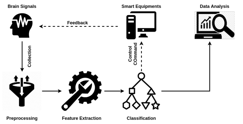
非侵入信号深度学习 工作流程包括几个关键部分:脑信号采集、信号预处理、特征提取、分类和数据分析
头骨让信号保真度为5%(以信噪比(SNR)衡量)
预处理:包含多个步骤,如信号清理(平滑噪声信号或解决不一致性)、信号标准化(沿时间轴对每个信号通道进行标准化)、信号增强(去除直流电)和信号压缩(呈现信号的简化表示)。
分类结果应用:神经疾病诊断、情绪测量和驾驶疲劳检测。
脑机接口的深度学习的分类:
传统BCI所面临的挑战:
大脑信号很容易被各种生物因素(如眨眼、肌肉伪影【肌肉产生的电波对脑电波的影响】、疲劳和注意力集中程度)和环境因素(如噪音)所破坏
深度学习好处:
深层神经网络和第二层神经网络都能捕获潜在的,具有代表性的特征。
综述论文贡献:
对非侵入性脑信号论文的全面性调查
功能性近红外光谱(functional near - infrared spectroscopy , fNIRS )【利用血液的主要成分对600-900nm近红外光良好的散射性,从而获得大脑活动时氧合血红蛋白和脱氧血红蛋白的变化情况,产生功能性神经影像】
综述论文内容:
讨论了流行的深度学习技术和最新的脑信号模型,为在给定特定信号亚类的情况下选择合适的深度学习模型提供了实用指南。
回顾了基于深度学习的脑信号分析的应用,并指出了一些有前景的未来研究课题。
基于信号收集方法的非侵入性脑信号分类(虚线不调查)
P300包含于ERP中。
ERP:一种特殊的脑诱发电位,通过有意地赋予刺激以特殊的心理意义,利用多个或多样的刺激所引起的脑的电位。它反映了认知过程中大脑的神经电生理的变化,也被称为认知电位,也就是指当人们对某课题进行认知加工时,从头颅表面记录到的脑电位。
其他脑成像技术(fNIRS,fMRI)中的视觉/听觉任务未曾有采用过深度学习,但理论上可行。
第三节,概述常用的深度学习模型
分类模型:Multi-Layer Perceptron (MLP) , Recurrent Neural Networks(RNN) , Convolutional Neural Networks (CNN) --> 特征提取和分类
表示模型:Autoencoder(AE), Restricted Boltz-mann Machine (RBM) , Deep Belief Networks(DBN) --> 只能特征提取
生成模型:Variational Autoencoder (VAE),Generative Adversarial Networks (GANs) --> 主要用于生成脑信号样本,增强训练集
各个非侵入式脑信号特征:
第四节,最先进的脑信号深度学习技术
4.1.1.1 睡眠脑电:
主要用于识别睡眠阶段、诊断睡眠障碍或培养健康习惯
睡眠阶段包括清醒、非快速眼动1、非快速眼动2、非快速眼动3、非快速眼动4和快速眼动。
美国睡眠医学学会(AASM)建议将睡眠分为五个阶段:清醒、非快速眼动1、非快速眼动2、慢波睡眠(SWS)和快速眼动。
识别睡眠阶段,一般通过滤波器实现脑电信号的预处理,数据通常是30s的窗口,50hz。
分类模型:CNN用于单通道EEG的睡眠阶段分类,86%精确度
表示模型:DBN-RBM(深度置信网络-受限玻耳兹曼机)从睡眠脑电信号中提取功率谱密度 (PSD,表示随机信号的强度),在局部数据集达到F-1值92.78%(兼顾召回率和精确度)
4.1.1.2 运动想象脑电:
深度学习在运动想象脑电图和真实运动脑电图的分类上显示出优越性
分类模型:大多使用CNN来识别脑电图,例如:
从EEG信号中学习情感信息,构建改进的LSTM控制智能家电
4.1.1.3 情绪脑电图
个体的情绪可以从三个方面来评价:评价值(积极感情的值)、唤起度(激动的程度)和控制力 。
这三个方面的结合形成了恐惧、悲伤和愤怒等情绪,这些情绪可以通过脑电图信号来揭示。
分类模型:传统上使用MLP,CNN和RNN正在越来越流行
通过多通道脑电信号转化为二维矩阵来捕捉通道之间的空间相关性
4.1.1.4 精神病脑电图
大量研究人员利用脑电图信号诊断神经系统疾病,特别是癫痫发作
分类模型:CNN广泛应用于癫痫发作的自动检测
CNN对癫痫发作的高通量(1hz)EEG信号进行研究,获得了94.7%的AUC
在抑郁症检测上采用了13层CNN模型,在30名受试者的局部数据集上进行了评估,基于左半球和右半球EEG信号的准确率分别为93.5%和96.0%
4.1.1.5 数据增强
实验1:EEG信号转换为图像
首先证明了脑电波中包含的信息被赋予了区分视觉对象的能力
然后使用RNN提取了更健壮、更具区分性的脑电数据表示。
最后,利用GAN范式训练了一个由学习的EEG表示调节的图像生成器,该生成器可以将EEG信号转换为图像
实验2:将EEG信号转换为图像
当受试者观察屏幕上的图像时,采集脑电图信号。将脑电信号的潜在结构作为输入,提取脑电信号的潜在特征。
GAN的产生器和鉴别器均由卷积层构成。该发生器根据训练后的脑电信号生成图像。
实验3:癫痫发作数据增强的GAN(生成式对抗网络)
作者证明了GAN优于其他生成模型,如AE和VAE(可变自动编码器)。增强后,分类准确率从48%提高到82%。
4.1.1.6 其他
实验1:听觉/视觉刺激(持续存在的刺激)如何影响脑电图信号
13名受试者受到23种节律性刺激的刺激,其中包括12种东非和12种西方刺激。
对于24类分类,提出的CNN平均准确率为24.4%。
之后,作者利用卷积AE进行表征学习,CNN用于识别,12类分类的准确率达到27%
实验2:区分是在听歌还是想象歌曲
提出两个深度学习模型,使用二值分类任务,所提出的CNN和DBN-RBM(三个RBM)的准确率分别为91.63%和91.75%。
实验3:自发脑电图可以用来区分使用者的心理状态(逻辑与情绪)
实验4:认知负荷(处理具体任务时加在学习者认知系统上的负荷)或体力负荷对EEG的影响
实验5:在不同心理负荷下,受试者之间及受试者本身中的一般特征是恒定的。
脑电信号经低通滤波器滤波后,转换到频域,计算功率谱密度(PSD)。
提取的PSD特征被输入到去噪D-AE结构中,以便于进一步的细化。最终得到了95.48%的准确率。
实验6:驾驶员疲劳检测 --- 三维CNN
实验7:驾驶员疲劳检测 --- ICA+DBN-RBM
达到85%左右准确率,二分类(“昏昏欲睡”或“警惕”)。
实验8:驾驶员疲劳值检测 --- DBM-RBM+SVM,精度达到73.29%
实验9:调查了不同低负荷水平下驾驶员的心理状态。提出了一种基于脑电信号直接检测驾驶负荷的CNN方法。
实验10:基于EEG信号的眼睛状态(闭或开)的检测
三个RBM的DBN-RBM和三个AEs的DBN-AE,98.9%的高准确率
事件相关去同步(ERD)表示正在进行的EEG信号的功率下降,
事件相关同步(ERS)表示EEG信号的功率增加
实验11:采用CNN在观看特定视频时通过脑电图检测学校欺凌行为。
实验12:结合RNN和CNN提出了一个级联框架来预测个体的情感水平和个人因素(五大人格特征、情绪和社会背景)。
实验13:试图根据使用者的脑电图信号来识别他们的性别
采用标准的CNN算法,在局部数据集上实现了81%的二元分类精度
实验14:驾驶员的脑电图信号可以区分刹车意图和正常驾驶状态
**实验15:**将大脑信号和推荐系统结合起来,通过EEG信号预测用户的偏好。
共有16名受试者接受了60个手镯状物体作为旋转视觉刺激物(3D物体)时采集脑电信号的实验。
然后采用MLP预测用户喜欢或不喜欢。本次勘探的预测精度为63.99%。
**实验16:**试图探索一个可用于各种脑信号范式的共同框架,并评估鲁棒性。基于compact CNN的EEGNet [73]
4.1.2.1 ERP事件相关电位
在大多数情况下,ERP信号都是通过P300现象来分析的。
4.1.2.1.i VEP视觉诱发电位
较热门。
实验1:通过深度学习提取具有代表性的特征来研究运动开始的 VEP(mVEP)
压缩后的信号被发送到DBN-RBM算法中,以获取更抽象的高层特征。
实验2:P300信号特征提取
通过带通滤波器(2∼35hz)过滤视觉刺激的P300信号,
该模型包括一个2D CNN来捕获空间特征,然后在LSTM层中进行时间特征提取。
实验3:使用AE模型进行特征提取,然后使用支持向量机分类器。
实验中,每一段包含150个点,分为五个时间步,每一步有30个点。
实验4:DBN-RBM代表性模型与支持向量机分类器相结合进行隐藏信息测试(??),97.3%准确率
实验5:提高P300写字机准确率
一种基于CNN的新模型,该模型包括5个具有不同特征集的低层CNN分类器
第三届BCI竞赛数据集II中,最高准确率达到95.5%
4.1.2.1.ii AEP听觉诱发电位
较少研究。
实验1:提出并测试了18个CNN结构来对单次试验的AEP信号进行分类。
实验分析表明,无论卷积层数多少,CNN框架都能有效地提取时空特征。
4.1.2.1.iii RSVP快速连续视觉表示
CNN和MLP在这里取得一定成功。
实验1:一种针对RSVP的主题间和任务间检测的CNN模型。
实验结果表明,CNN在交叉任务中表现良好,但在跨主题情境下表现不佳。
实验2:比较了三种不同的深度神经网络算法,以预测受试者是否看到了目标。
MLP、CNN和DBN模型的AUC分别为81.7%、79.6%和81.6%。
...
4.1.2.2 SSEP稳态诱发电位
大多数研究稳态视觉诱发电位(SSVEP),指由闪烁的视觉刺激引起的脑震荡,通常产生于顶叶和枕叶。当施加一个恒定频率的外界视觉刺激时,与刺激频率或谐波频率相一致的神经网络就会产生谐振,导致大脑的电位活动在刺激频率或谐波频率处出现明显变化,由此产生SSVEP信号。
实验1:寻找SSVEP的中间表现形式。
提出了一种结合CNN和RNN的混合方法,直接从时域中提取有意义的特征,准确率达到93.59%。
实验2:紧凑CNN直接处理原始结果
实验3:采用了一种典型的稀疏AE模型,从多频视觉刺激中提取SSVEP的不同特征。
该模型采用了一个softmax层进行最终分类,准确率为97.78%。
...
4.2 fNIRS功能性近红外光谱
较少研究。
定义:利用血液的主要成分对600-900nm近红外光良好的散射性,从而获得大脑活动时氧合血红蛋白和脱氧血红蛋白的变化情况,产生功能性神经影像。
实验1:基于fNIRS信号分析了两种心理任务(心算和休息)之间的差异。
从前额叶皮层fNIRS中手动提取了6个特征,并比较了6个不同的分类器。
结果表明,MLP的准确率为96.3%,优于所有传统的分类器,包括SVM、KNN、naivebayes等。
实验2:试图通过fNIRS信号检测受试者的性别。
作者使用三层隐层去噪D-AE来提取显著特征并输入MLP分类器进行性别检测。
该模型在本地数据集上进行了评估,平均准确率为81%
相比fMRI信号,fNIRS具有更高的时间分辨率和更经济的价格
4.3 fMRI功能性磁共振成像
利用磁振造影来测量神经元活动所引发的血液变化。从而监测大脑活动
该领域,近年用了不少深度学习方法,特别是认知功能障碍的诊断上。
分类模型中,CNN是一种很有前途的fMRI分析模型
实验1:根据功能磁共振成像(fMRI)和核磁共振成像(MRI)数据,应用深层CNN识别阿尔茨海默病。
实验2:利用一种新的CNN算法建立了一种基于fMRI的脑肿瘤分割方法,它可以同时捕获全局特征和局部特征
实验3:采用CNN模型处理脑瘤患者的功能磁共振成像(fMRI)进行三类识别(正常、水肿或活动性肿瘤)。在BRATS数据集上对模型进行了评估,得到了88%的F1分数
实验4:利用CNN进行特征提取。提取的特征用支持向量机分类,用于癫痫发作的检测
大量文章证明了表示模型在识别功能磁共振成像数据方面的有效性。
实验1:利用一个由三个RBM分量组成的DBN-RBM从ICA处理的fMRI中提取显著特征,最终在四个公共数据集上实现了90%以上的F1平均测量值。
实验2:DBN-RBM和DBN-AE检测阿尔茨海默病
实验3:应用D-AE模型从静止状态的fMRI数据中提取潜在特征,用于诊断轻度认知功能障碍(MCI)。-
将潜在特征输入支持向量机分类器,识别率达到72.58%。
自然图像的重建引起广泛的关注。
实验1:从fMRI中重建视觉刺激的深卷积GAN,
发生器包含四个卷积层,以便将输入的fMRI转换为自然图像。
用于测量由大脑中神经元的电活动引起的磁场。通过磁变化反映大脑活动
实验1:致力于通过去除诸如眨眼和心脏活动等伪影来细化MEG信号。
最后,该方法在局部数据集上的灵敏度达到85%,特异性达到97%。
实验2:目标同实验1
基于深度学习的大脑信号系统主要用于检测和诊断精神疾病,如睡眠障碍、阿尔茨海默病、癫痫发作等。
睡眠障碍:
对于睡眠障碍的检测,大多数研究都集中在基于睡眠自发脑电图的睡眠阶段检测上。DBN-RBM和CNN被广泛应用于特征选择和分类。
阿尔茨海默病:
功能磁共振成像在阿尔茨海默病的诊断中有着广泛的应用。优点是高空间分辨率,几项研究的诊断准确率均在90%以上。
癫痫:
癫痫发作的检测主要基于自发脑电图。流行的深度学习模型包括独立的CNN和RNN,以及结合RNN和CNN的混合模型
例如,将D-AE应用于特征提取,然后将支持向量机应用于癫痫诊断
研究人员已经证明了深度学习模型在检测大量精神疾病方面的有效性,如抑郁症[113]、发作间期癫痫放电(IED)[230]、精神分裂症[211]、克雅氏病(CJD)[123]和轻度认知障碍(MCI)
随着物联网的发展,越来越多的智能环境可以连接到大脑信号。
例如,辅助机器人可用于智能家居,其中机器人可以由个体的大脑信号控制。
基于视觉刺激的自发EEG和fNIRS信号的机器人控制问题。
P300 speller,深度学习模型使大脑信号系统能够从非300片段中识别出P300片段
使用一种结合RNN、CNN和AE的混合模型,从MI-EEG中提取信息特征来识别用户想要说的字母。
应用于身份识别和身份验证
前者通过多类别分类来识别一个人的身份[6]。后者进行二元分类来决定一个人是否被授权
个性化信息(如多媒体内容)检索或智能人机界面设计
试图根据脑电图信号,使用深度学习算法(如CNN及其变体)将用户的情绪状态分为两类(积极/消极)或三类(积极、中性和消极)
DBN-RBM是从情绪自发脑电图中发现隐藏特征的最具代表性的深度学习模型
一般情况下,如果驾驶员的反应时间小于0.7秒,则认为驾驶员处于警戒状态;如果反应时间大于2.1秒,则认为驾驶员处于疲劳状态。
目前,基于EEG的驾驶困倦可以得到较高的识别率(82%∼95%)
适当的心理负荷对于维持人类健康和预防事故是必不可少的。
持续脑电来评估操作者的心理负荷,以警告随着时间,操作者的性能下降。
通过一个循环卷积框架研究了跨多个心理任务的心理负荷测量。该模型同时从空间、频谱和时间维度学习脑电特征,二值分类(高/低负荷水平)的准确率为88.9%
推荐系统,紧急刹车,视觉对象识别,内疚测试,隐藏信息测试,区分性别。
https://en.wikipedia.org/wiki/Self-driving_car https://physionet.org/physiobank/database/sleep-edfx/ https://massdb.herokuapp.com/en/ https://physionet.org/pn3/shhpsgdb/ https://physionet.org/pn6/chbmit/ https://www.isip.piconepress.com/projects/tuh.eeg/html/downloads.shtml https://physionet.org/pn4/eegmmidb/ http://www.bbci.de/competition/ii/ http://www.eecs.qmul.ac.uk/mmv/datasets/amigos/readme.html http://bcmi.sjtu.edu.cn/seed/download.html https://www.eecs.qmul.ac.uk/mmv/datasets/deap/ https://owenlab.uwo.ca/research/the.openmiir.dataset.html http://adni.loni.usc.edu/data-samples/access-data/ https://www.med.upenn.edu/sbia/brats2018/data.html
第六节,分析和指南,根据大脑信号选择适当的模型
70%的EEG论文关注自发EEG(133种出版物)。自发的脑电图分成几个方面:睡眠、运动想象、情绪、精神疾病、数据增强和其他 。
睡眠:总共19篇,6篇使用CNN,2篇RNN,还有3种RNN+CNN的混合模型。
运动想象:广泛使用CNN和基于CNN的混合模型。表示型模型常用DBN-RBN提取潜在特征。
情绪:总共25篇,超过一半使用表示模型(D-AE,D-RBM,DBN-RBM)。最典型的状态识别工作将用户的情绪识别为积极、中立或消极。进一步对配价和唤起率进行分类
精神疾病:大部分相关研究集中在癫痫发作和阿尔茨海默病的检测上。大部分相关研究集中在癫痫发作和阿尔茨海默病的检测上。许多研究可以达到90%以上的高准确率。在这一领域,标准的CNN模型和D-AE是普遍存在的。一个可能的原因是CNN和AE是最著名和最有效的深度学习模型的分类和降维
数据增强:基于GAN的数据扩充
其他:大约有30个研究正在调查其他自发脑电图,如驾驶疲劳、视听刺激冲击、认知/心理负荷和眼睛状态检测。这些研究广泛应用标准CNN模型和变体。
视觉诱发电位(VEP)引起大量研究(21篇)。6种混合模型。
快速连续视觉表示(RSVP),只有CNN算法。
fNIRS图像的研究很少采用深度学习的方法,主要的研究只是采用简单的MLP模型。我们认为,由于fNIRS具有高便携性和低成本的特点,应引起更多的关注。
至于功能磁共振成像,有23篇论文提出了深度学习的分类模型。CNN模型因其在图像特征学习中的突出表现而被广泛应用。
6.2 深度学习模式的选择标准
结论1:大多数采用判别模型。
结论2:超过70%的判别性模型都采用了CNN及其变体,为此我们提供了以下原因:
首先,CNN的设计足够强大,能够从EEG信号中提取潜在的鉴别特征和空间相关性 进行分类。因此,有些研究采用CNN结构进行分类,而有些研究则采用CNN结构进行特征提取。
CNN在一些研究领域(如计算机视觉)取得了巨大的成功,更容易找到代码。
一些脑信号图(如功能磁共振成像)是自然形成的二维图像,有利于CNN进行处理。
结论3:表示模型中,DBN,尤其是DBN-RBM是最常用的特征提取模型。原因有二:
【大多数采用DBN-RBM模型的作品都是在2016年之前出版的。可以推断,在2016年之前,研究人员更倾向于使用DBN进行特征学习,然后使用非深度学习分类器;但最近,越来越多的研究希望采用CNN或混合模型进行特征学习和分类。】
结论4:生成模型很少独立使用,基于GAN和VAE的数据增强和图像重建主要集中在fMRI和EEG信号上,有前途。
结论5:53篇论文中,RNN和CNN的组合约占五分之一,结合后具有很好的时空特征提取能力。
结论6:表示模型+判别模型也很常用,28篇中有这种方法,所采用的表示模型多为AE或DBN-RBM,同时所采用的判别模型多为CNN。
将脑信号分析应用于医疗领域是目前最吸引人和最热门的领域。
一般来说,大多数深度学习算法在多个睡眠阶段场景下都能达到85%以上的准确率。
对于fMRI图像,CNN在网格化空间信息学习方面具有很大的优势,使其获得了非常全面的分类准确率(90%以上)。
至于癫痫发作,一般是根据脑电图信号进行诊断。单一的RNN分类器(如LSTM或GRU)由于其良好的时间依赖性表示能力,似乎比其对应的分类器工作得更好。
检测阿尔茨海默病的一个关键方法是通过测量大脑特定区域的功能来分析大脑信号。具体来说,可以通过自发的脑电图信号或功能磁共振成像来进行诊断
由于视觉诱发电位明显且易于检测,许多研究都集中在VEP信号上。一个重要的数据来源是来自第三届BCI竞赛。
脑电信号具有较高的时间分辨率,能够捕捉快速变化的情绪。因此,几乎所有的研究都是基于自发的脑电信号。这些信号是在被试观看视频时收集的,视频被认为是激发受试者特定情绪的。主要是使用层次化CNN,DBN-RBM结合强分类器,前一种更好。
一般框架需要两个关键能力:注意机制和捕捉潜在特征的能力。前者保证了框架能够集中于输入信号中最有价值的部分,而后者使框架能够捕捉到与众不同和信息丰富的特征。
方法2:CNN是最适合捕捉不同层次和范围特征的结构。未来,CNN可以作为一种基本的特征学习工具,并与适当的注意机制相结合,形成一个通用的分类框架。
方法1:可以考虑如何解释由深层神经网络导出的特征表示,学习的特征与任务相关的神经模式或精神障碍的神经病理学之间的内在关系。
方法1:实现这一目标的一个可能的解决方案是建立一个个性化的迁移学习模型 。
个性化情感模型可以采用转换参数传递的方法来构造个体分类器,并学习映射数据分布和分类器参数之间关系的回归函数
方法2:从输入数据中挖掘与主题无关的组件。输入的数据可以分解为两部分:一个依赖于主题的主题相关组件和一个所有主题都通用的主题无关组件。一个混合多任务模型可以同时处理两个任务,一个侧重于人的识别,另一个侧重于类识别。在类识别任务中,需要一个训练良好、收敛良好的模型来提取与主题无关的特征。
Adversarial V ariational Embedding (对抗性变异嵌入)-----> 高质量生成模型
有两种方法可以增强无监督学习:
一种是利用众包(给大众志愿者)方法对未标记的观测值进行标记;
另一种是利用无监督域自适应学习,通过线性变换来调整源脑信号和目标信号的分布
在真实场景中,大脑信号系统需要接收实时的数据流并实时产生分类结果
由于受试者注意力不集中和设备固有的不稳定性(例如采样率波动)等诸多因素,采集到的实时信号更具噪声和不稳定性。通过我们的实验,在线脑信号系统的准确率通常比同类系统低10%。
方法:投票和聚合来平均多个连续样本的结果,提高解码性能。
脑电采集设备主要有三种:不便携头戴式、便携式头戴式和耳式脑电传感器。
第一种,采样频率高,信道数多,信号质量高,但价格昂贵。适合医院体检。
第二种,(例如Neurosky、Emotiv EPOC),有1∼14个通道和128∼256采样率,但读数不准确,长期使用后会造成不适。
第三种,还在实验室阶段。EEGrids是唯一商业化的耳脑电设备。
受限玻尔兹曼机 RBN (2000年后流行)
RBM可以看做是一个编码解码的过程,从可见层到隐藏层就是编码,反之是解码。对于每个训练样本, 期望编码解码后的可见层输出和之前可见层输入的差距尽量的小。
RBM详细推导过程:https://www.cnblogs.com/pinard/p/6530523.html
深度波尔茨曼机Deep Boltzmann Machine (DBM)
RBN实现的深度置信网络 (DBN-RBN)
与DBM的区别是隐藏层之间为单向的。优化计算更简单。
降噪自编码器(D-AE)
DAE(Denoising Autoencoder)的核心思想是,一个能够从中恢复出原始信号的神经网络表达未必是最好的,能够对“损坏”的原始数据编码、解码,然后还能恢复真正的原始数据,这样的特征才是好的。
卷积神经网络(CNN)
循环神经网络(RNN)
长短期记忆(LSTM)
评价标准
一种JSSP的DRL环境 作者使用单智能体和多智能体来划分目前DRL方法的两大类
多智能体:2018 DQN,2020 DDPG效果更好
单智能体:2020 GNN+MLP,2020 CNN(处理时间,时间表,机器利用率)+DRL,2019 DQN+Rule
使用标准的JSSP文件(txt)方式读写,样例可看困惑点2
一个二维数组solution,若是-1表示没排,否则为开始运行的时间步
离散集合={Job是否加工-J$_i$,空闲状态},机器选择行为,行为对应作业和空闲
因此,对于每个Job而言,需要完成|M|个行为(机器的数量)。每个行为表示Job在每台机器上的加工时间,如果不需要在该机器上执行,可以当作一个0?
对于每个机器而言,需要运行至少|J|个与job有关的行为,加上若干个no-op(空闲)操作。
该函数相对于makespan能得到更紧密的解。
不用执行到最后一步,就能获得一个局部reward。
makespan可以看成是全局p+empty,而这里是局部的p-empty,那么改变之处在于系数-1和全局变为局部。
作者新建自己环境的代码十分受用,让我对新建gym的环境有了一个详细的了解
wandb和ray两个库的使用具有一定的启发,但可能更适合较大的项目
第四页中的问题对称性,讲述了一些JSS问题的对称性,通过破坏对称性,而降低搜索解空间的大小
同一时间步长中,操作具有对称性,也就是操作的执行顺序待定。怎么解决?以及为什么说直接赋予机器从小到大的索引会导致失去全局视图。
同一机器中,"运行"操作和"无运行"操作具有对称性,也就是op和no-op两者的执行顺序待定。解决方案:当no-op时,其他的操作临时设未不可执行。以及通过非最终状态优先调度的规则。
复现代码时候遇到的问题(已解决,记录):
'env': 'JSSEnv:jss-v1',该环境已经创建好并上传gym库中,作者使用的ray库会自动生成一个包含该环境名字的本地日志。而windows文件不允许冒号,所以需要修改ray库的底层代码中的日志文件名字生成方式。
大体分三块
强化学习环境:已经注册成gym库的环境,各种强化学习包都可以用。
CP.py:是使用OR tools的求解器,进行求解的方法,能达到比较好的解。
mian.py:使用ray中的PPO算法,只修改了一个全连接层,然后定义了一些参数,就可以使用作者的环境来训练。
其他读后感主要写在代码注释中,目前均已跑通。
y u i = { 1 , i f i n t e r a c t i o n i s o b s e r v e d ; 0 , e l s e y_{ui}= \begin{cases} 1,\ if\ interaction\ is\ observed;\\0,\ else \end{cases} y u i = { 1 , i f in t er a c t i o n i s o b ser v e d ; 0 , e l se Scheduling 用于发布个人阅读深度强化学习+Scheduling领域的读后感
Pytorch 目前根据官网教程和《动手学习深度学习》pytorch版学习
Deep Learning 主要根据《神经网络与深度学习》书籍进行读书笔记,其中部分截图上传到github图床,需要翻墙才能正常阅读.
1.2自动梯度
复制 # 设置跟踪向量
x = torch.ones(2, 2, requires_grad=True)
print(x)
复制 tensor([[1., 1.],
[1., 1.]], requires_grad=True)
复制 tensor([[3., 3.],
[3., 3.]], grad_fn=<AddBackward0>)
复制 Help on AddBackward0 object:
class AddBackward0(object)
| Methods defined here:
|
| __call__(self, /, *args, **kwargs)
| Call self as a function.
|
| name(...)
|
| register_hook(...)
|
| ----------------------------------------------------------------------
| Data descriptors defined here:
|
| metadata
|
| next_functions
|
| requires_grad
复制 z = y * y *3 # z = (x+2)^2 *3
out = z.mean() # out = (x+2)^2 *3/4
z, out
复制 (tensor([[27., 27.],
[27., 27.]], grad_fn=<MulBackward0>),
tensor(27., grad_fn=<MeanBackward0>))
复制 a = torch.randn(2, 2)
a = ((a*3)/ (a-1))
# 默认为Flase
print(a.requires_grad)
# 设置梯度为True
a.requires_grad_(True)
print(a.requires_grad)
b = (a*a).sum()
print(b.grad_fn)
复制 False
True
<SumBackward0 object at 0x7fd230a89d90>
复制 # 求出out对x在x=1的偏导数
out.backward()
x.grad
复制 tensor([[4.5000, 4.5000],
[4.5000, 4.5000]])
复制 x = torch.randn(3 , requires_grad=True)
y = x *2
# norm是求L2范数,平方之和而后开方
while y.data.norm() < 1000:
y = y *2
print(y)
复制 tensor([ 277.2757, 3.3198, -986.0908], grad_fn=<MulBackward0>)
复制 v = torch.tensor([0.1, 1.0, 1.0], dtype=torch.float)
# 将向量v传递给backward
y.backward(v)
# 计算向量-雅可比积,也就是在x=v的时候的梯度
x.grad
# 下面表示2^11次方
复制 tensor([ 204.8000, 2048.0000, 2048.0000])
复制 print(x.requires_grad)
print((x ** 2).requires_grad)
# 取消求梯度
with torch.no_grad():
print((x ** 2).requires_grad)
复制 print(x.requires_grad)
# 取消求梯度
y = x.detach()
print(y.requires_grad)
print(x.eq(y))
复制 True
False
tensor([True, True, True]) 大多基于静态数据上,无法对快速变化的大脑信号进行准确分类【最先进的多类别运动图像脑电图分类准确里低于80%】
功能性磁共振成像(FMRI,functional magnetic resonance imaging)【是一种新兴的神经影像学方式,其原理是利用磁振造影来测量神经元活动所引发的血液变化。从而监测大脑活动】
脑磁图(Magneto Encephalo Graphy,MEG)【是一种非侵入性技术,用于测量由大脑中神经元的电活动引起的磁场。通过磁变化反映大脑活动】
CNN+MLP来预测睡眠阶段
MLP接收经短时傅立叶变换(STFT)处理的0.5~32hz的频谱信号。
CNN+LSTM的睡眠阶段自动评分模型、
前者用于发现”time-invariant dependencies“
先用CNN捕获潜在的连续特征,然后应用弱分类器选择重要特征进行最终分类
研究CNN如何通过MI EEG样本序列来表示光谱特征
另外,还有MLP分类(前期对EEG相位【波峰,波谷】特征敏感,后期对EEG幅度特征敏感)
表示模型:DBN具有很高的代表性,被广泛应用,例如:
利用离散小波变换对脑电信号进行处理,然后应用基于声发射去噪的DBN-AE
遗传算法(用于超参数调整)和MLP(用于分类)的组合
混合模型:
利用CNN从EEG信号的时间、频域和位置信息中提取高级表示,然后使用一个包含7个AEs的DBN-AE作为分类器
使用去噪AE进行降维,将multi-view CNN与RNN相结合,在公共数据集上实现了对潜在时空信息的发现,平均准确率为72.22%。
时空递归神经网络:利用多向RNN层来发现长距离上下文线索,使用双向RNN层来捕获先前空间RNN产生的序列特征
表示模型:DBN-RBN因为情感识别的无监督表示能力强而广泛使用
用三个RBM和一个RBM-AE的DBN-RBM算法来预测情感状态
将DBN-RBM与SVM和隐马尔可夫模型(HMM)相结合来预测情感状态
提出五个隐层的D-RBM算法,用于情感识别中重要的频率模式(??)和信息通道(了解情感的渠道)的搜索
首先剔除高误差通道,然后根据剩余通道的代表性特征,采用D-RBM方法进行情感状态识别
双模深度自动编码器(BDAE)来研究男性和女性的情绪模式差异,该模型同时接收EEG和眼球运动特征,并在融合层中共享信息,该层与支持向量机分类器相连接。
结果:女性在恐惧情绪上具有较高的脑电信号差异性,而男性在悲伤情绪上具有较高的差异性。
跨个体 (克服不同受试者或不同实验阶段采集的样本之间的不匹配分布):结合AE和子空间对齐方法,提出了一种无监督域自适应技术,称为子空间对齐自动编码器(SAAE)。在独立场景下,该方法的平均准确率为77.88% 。[94]
混合模型:常用的是RNN+MLP
采用LSTM架构从情绪EEG信号中提取特征,并将特征转发到MLP中进行分类
多视角集成分类器,利用多模态生理信号识别个体情绪。集成分类器包含多个D-AEs(去噪自编码器?),具有三个隐藏层和一个融合结构。
然后将D-AE的输出发送到由另一个D-AE组成的融合结构
结合DBN-RBM有效特征提取和MLP进行分类,实现了一个情感识别系统
利用CNN结构提取多通道EEG信号的合适特征,将阿尔茨海默病从轻度认知障碍患者和健康对照组中进行分类
回声状态网络(ESNs)模型,它是RNN的一个特殊类别,用来区分RBD和健康个体
眼运动行为障碍(RBD)可引起帕金森病(PD)等多种精神障碍疾病
使用CNN提取潜在特征,并输入随机森林分类器,以最终检测新生儿癫痫发作
表示模型:对于疾病检测,一种常用的方法是采用具有代表性的模型(例如DBN),然后使用softmax层进行分类
采用DBN-AE从癫痫发作的EEG信号中提取信息特征。将提取的特征输入到传统的logistic回归分类器中进行癫痫检测。
多视图DBN-RBM结构来分析抑郁症患者的EEG信号。
该方法包含多个输入通路,由两个RBM组成,每个通路对应一个EEG通道。
所有的输入路径将合并成一个由另一个RBMs组成的共享结构。
混合模型:一种流行的混合方法是RNN和CNN的结合
研究了CNN-LSTM在信道选择后检测癫痫的性能,灵敏度(实际真,结果真)在33%到37%之间,而假警报(实际假,测出真)在38%到50%之间。
通过整合时间和空间信息来自动解释EEG。二维和一维cnn捕捉空间特征,LSTM网络捕捉时间特征。
将D-AE和MLP结合起来。
首先用0.5∼70hz的带通滤波后,将其送入具有两个隐藏层的D-AE中进行特征表示。
最后,在局部数据集上,MLP分类器的准确率达到81∼83%。
卷积自动编码器,用卷积和去卷积层代替标准声发射中的完整连接层,以无监督的方式提取癫痫特征
从时间采样、通道批量和窗口采样三个层面对DBN-RBM进行了评估。实验表明,通道批量的性能优于其他两级。
大脑信号控制的外骨骼可以帮助那些在行走和日常活动中损坏下肢运动系统的残疾人。
其他一维信号(如EEG)可以转换成二维图像,供CNN进一步分析。转换方式如下:
1)将每个时间点转换为二维图像;假设我们有32个通道,我们可以在每个时间点收集32个元素(每个元素对应于一个通道)。收集到的32个元素可以根据空间位置转换为二维图像。
2)将一个片段转换为二维矩阵。假设我们有32个通道,段包含100个时间点。所收集的数据可以被安排为一个形状为[32,100]的矩阵
CNN使用:
只有20%的基于判别模型的论文采用RNN,这远远低于我们的预期,因为RNN在时间特征学习方面表现出了强大的能力。造成这种现象的一个可能原因是RNN对长序列的处理非常耗时,而且脑电信号通常是长序列
MLP算法由于其简单的深度学习结构,其有效性(如非线性能力)不如其他算法,因而不受欢迎。
学习视频:https://www.bilibili.com/video/BV1dt411U7ad?from=search&seid=10143340215037418101
F1值
每到一个时间步(可以定义为1秒或者1分),每台机器进行一个行为选择
最终优先级:如果该Job已分配的行为数量等于|M|-1,说明最后一个动作已经确定了要在哪里执行。
奖励函数:作者定义了一个schedule area,在这区间内计算reward,可以获得更多个奖励函数,从而为强化学习使用。
ray能够快速使得模型快速落地,并变成分布式,相比较spark更简单,更便捷
之后打算:
进一步看懂代码,模型代码很少,基本已看完,但环境的代码很复杂,还没看完。
先使用pytorch替换掉里面的ray的ppo模型,然后逐步调试,理解环境部分的代码
似乎JSSP问题是每个Job在每台机器上都有执行一定时间,还是说我看到的刚好是特例?
R ( s , a ) = p a j − ∑ m ∈ M empty m ( s , s ′ ) p a j 是作到某个时刻的已排程时间总和 a 表示当前行为 , s 表示当前状态 , s ′ 表示下一个状态 e m t p t y m ( s , s ′ ) 是计算机器 m 在两个状态之间的 i d l e 时间 在实现的代码中,作者将所有的 R 都除以一个最大的工序加工时间来达到缩放 R(s, a)=p_{a j}-\sum_{m \in \mathcal{M}} \operatorname{empty}_{m}\left(s, s^{\prime}\right) \\ p_{aj}是作到某个时刻的已排程时间总和\\ a表示当前行为,s表示当前状态,s^{\prime}表示下一个状态 \\ emtpty_{m}(s, s^{\prime})是计算机器m在两个状态之间的idle时间\\ 在实现的代码中,作者将所有的R都除以一个最大的工序加工时间来达到缩放 R ( s , a ) = p aj − m ∈ M ∑ empty m ( s , s ′ ) p aj 是作到某个时刻的已排程时间总和 a 表示当前行为 , s 表示当前状态 , s ′ 表示下一个状态 e m tpt y m ( s , s ′ ) 是计算机器 m 在两个状态之间的 i d l e 时间 在实现的代码中,作者将所有的 R 都除以一个最大的工序加工时间来达到缩放
心理学随机森林 用机器学习(即随机森林):
关系质量的最高预测因子是:(RF里的重要性?)
个体差异最大的预测因子:(方差?)
??特定于关系的变量在基线时 预测的方差高达45%,在每个研究结束时预测的方差高达18%。
Overall, relationship-specific variables predicted up to 45% of variance at baseline, and up to 18% of variance at the end of each study.
??个体差异和伴侣报告除了行为人报告的关系特异性变量外,没有预测效果。
Importantly, individual differences and partner reports had no predictive effects beyond actor-reported relationship- specific variables alone.
结论:
所有个体差异和伴侣经验的总和通过一个人的特定关系经验对关系质量产生影响 ,并且由于个体差异的调节和伴侣报告的调节而产生的影响可能很小 。
??最后,通过任何自我报告变量的组合,发现关系质量的变化 (即,在研究过程中关系质量的增加或减少)在很大程度上是不可预测的 。
已经确定了数百个据称影响浪漫关系质量的变量 。目前的项目使用机器学习来直接量化 和比较11196对浪漫夫妇中许多这样的变量的预测能力 。
人们对关系有自己的判断,比如他们对伴侣的满意程度 和忠诚程度 ,感激程度 ,解释了他们目前满意度的45%。
建立分类树和回归树
随机森林方法使用一个随机的预测器和参与者子集 ,通过一个称为递归分区 的过程,一次一个地测试每个可用预测器的强度 。
举例能够预测非线性关系:
For example, a model with actor- and partner-reported predictors would detect any robust actor × partner interactions (e.g., moderation, attenuation effects, matching effects) that could not be captured in a model featuring actor- or partner-reported predictors alone.
参数设置:
ntree = 5000,树的数量
mtry = 1/3,每个节点上可用于拆分的预测因子数量
R语言中的VSURF包:An R Package for Variable Selection Using Random Forests Robin Genuer
输出:
每个模型都显示了模型解释的总方差量 ,以及作为预测变量的具体变量
模型设置:
对每个数据集进行了21个随机森林模型,
类似地,我们对每个包含忠诚 的数据集(即我们的次要因变量)进行了21个随机森林模型,每个数据集总共有42个随机森林模型(最大值)。
总共有43个数据集,每个数据集最大42个模型
每个数据集的结果在 https://osf.io/4pbfh/
42个模型中的每一个都作为一个??单独的随机效应元分析 进行了检验;
21个满意度荟萃分析分别包含k=43个效应量(effect sizes),每个数据集对应一个21个满意度模型
21个忠诚度元分析每个包含k=31个效应量。有31个数据集有忠诚数据,每个数据集对应一个21个忠诚度模型
满意度和忠诚度的元分析数据文件在https://osf.io/v5e34/。
调节分析Moderation Analyses
分析12种可能的元分析调节因子,
10个是数据集的特征:研究长度、时间点之间的长度、时间点的数量、样本的平均关系长度、样本的平均年龄、开始收集数据的年份、国家、出版状态(至少有1个出版物与未出版过的文献)、样本类型(社区与大学生)、关系状况(约会vs.已婚)。
使用了
初步荟萃结分析结果Primary Meta-Analytic Results
元分析调节Meta-Analytic Moderators
预测限制效应Predictor Restriction Effects
具体结构的预测成功Predictive Success of Specific Constructs
两个问题:
答案:
如果人们设法建立起一种以欣赏、性满足和较少冲突 为特征的关系,并且他们认为他们的伴侣是忠诚的和有反应的 ,那么这些个人的风险因素可能无关紧要。
关系质量可以从各种结构中预测,但有些结构比其他结构更重要,而最接近的预测因素是表征一个人对关系本身感知的特征。
P300数据学习 6次行,6次列,分别有一行和一列包含目标字符,此时引起的反应,类似P300
文件名:example.m
该程序比较session10-run01数据集中,对目标与非目标刺激(即,包含/未包含所需字符的刺激)的响应
文件名:testclass.m
使用一个非常简单的分类器来预测session12-run01中单词的第一个字符
它在增强后使用Cz和310ms处的一个样本进行分类。 它确定目标字符为振幅最高的字符(Cz / 310ms)
它针对session12中的单词01中的第一个字符执行此操作
肾透析移植机器学习 本文综述人工智能/机器学习(AI/ML)算法在肾替代治疗(血液透析,腹膜透析和肾移植)中的研究现状及其影响。
研究了三个医疗领域关于血液透析(hemodialysis,HD),腹膜透析(peritoneal dialysis,PD),肾移植(kidney transplantation,KT)的四个使用AI/ML的电子数据库或研究。
所以分为了HD,PD,KT三类。
AI能比肾脏学家更好的预测:体积,KT/V(一定透析时间内透析器对尿素的清除量与体积的比值。),透析期间发生低血压或心血管事件。
这些实验报告了AI/ML对G5D/T患者的生活质量和生存期的强大影响。
未来几年,人们可能会看到AI/ML设备的出现,它有助于透析患者的管理,从而提高生活质量和生存。
CKD: chronic kidney disease,慢性肾脏病
G5D/T: 终末期肾脏病,需要长期透析治疗。
FDA: US Food and Drug Administration,美国食品和药物监管局
ESRD: end-stage renal disease,终末期肾病患者
RCTs: randomized controlled trial,随机对照试验
AI/ML的方法已经步入平稳期: 美国食品和药物管理局发布了监管框架,用于修改基于AI/ML的软件作为医疗设备。该委员会去年批准了至少15个涉及医疗领域的人工智能/深度学习平台(例如,用于房颤检测、CT脑出血诊断、冠状动脉钙化评分、辅助中风诊断或乳房x线摄影乳房密度)。
有数据集但没成功: 在过去的15年里,许多问题和并发症产生的终末期肾病需要透析,使得人工智能算法得到了初始输入。但上述的成功案例均未发现。
成功案例引起肾学家思考 :医学图像处理对医疗保健的重大影响,手术中的智能机器人,苹果手表对心房颤动检测的影响。
思考 :
下一步目标 :用AI加强透析机(也就是人工肾)的功能。
理论基础 :2019年的论文——基于透析患者特征、历史血流动力学反应和透析相关处方,开发了一个多终点模型来预测特定时段的Kt/V、液体容量去除、心率和血压,
理论意义 :为关于ESRD患者的人工智能研究打开了大门,ml驱动的机器连续自主地改变参数(温度、透析液电解质成分、持续时间和超滤速率),避免透析过程中糟糕的情况(例如低血压)。从而告诉我们,肾脏学是一门“个体化医学”,因为透析过程不一样。
遵循PRISMA指导原则(详看上述专有名词)
搜索PubMed、SCOPUS、Web of Science和EBSCO的电子数据库,最早的论文为2019年8月。
筛选阶段获得77篇论文,通过两名审稿人讨论和协商后,69项符合标准。(对应表1-表3)
图1:筛选过程分为四个流程:
阅读题目和摘要后再剔除,189篇重复,68篇不是手稿(手写),7篇没有临床,13篇没有文本
图2:所有研究分为三大类,12小类:
注:他克莫斯移植后,而不是后移植,指治疗调节。
实验的特征 :
大多数研究是观察性的,除了一个随机对照实验(RCT),超过60%的研究是在2010年之后报道的。
大多数HD(血液透析)研究涉及个体化贫血管理和透析过程参数。准确预测移植排斥反应 或移植后个体化免疫抑制治疗 是AI和KT(肾透析)试验的主要主题。
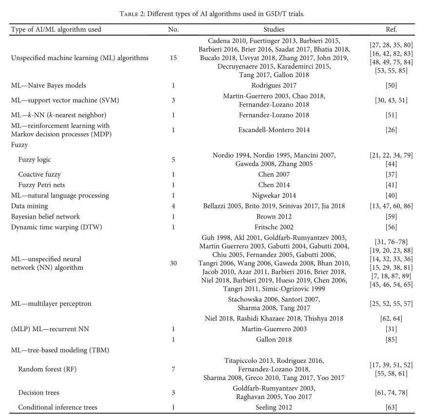
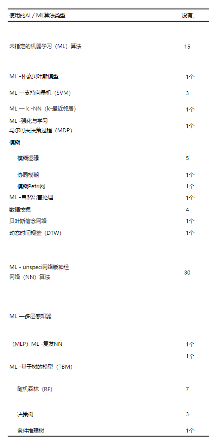
表2:根据AI算法的类型进行分类:
算法分析 :
64项研究包括ML算法: 未指定的、朴素贝叶斯模型、支持向量机(SVM)和马尔可夫决策过程强化学习 (MDP)。
1个K近邻,1个MLP,30个未指定的神经网络算法。
11项研究基于树的模型(TBM),随机森林(RF)或条件推理树
3.1.1 Key Message
人工智能如何改善向HD(血液透析)提供的医疗服务?
预防
人工智能能够为临床结果不令人满意的HD实验确定风险概况。
实验一
一个MLP模型使用了来自111名尿毒症患者5年PD数据库的透析前数据并证明了该方法将透析前患者分为高转运蛋白组和低转运蛋白组有效性。
可以为尿毒症患者提供更好的治疗选择,这将改善PD患者的预后,降低发病率和死亡率。
实验二
利用反向传播方法构造和训练了73-80-1节点结构的MLP,确定PD技术失败的相关因素,以便开发干预措施以减轻风险因素
3.2.1Key Message
人工智能的使用如何改善向PD(腹膜透析)提供的医疗服务?
预防
人工智能被用来确定PD技术失败的相关因素,指定干预措施以减轻风险因素
实验一
NNs可用于预测慢性肾移植排斥反应(作者描述了对27例慢性排斥反应患者的回顾性分析,八个简单变量对排斥反应有很大影响)
实验二
一项对2005年至2011年500名患者的研究使用最大似然算法(SVM、随机森林和离散余弦变换)预测“延迟移植功能”,结果表明线性SVM具有最高的鉴别能力(AUROC为84.3%),优于其他方法。
3.3.1Key Message
人工智能的使用如何改善向KT提供的医疗服务?
诊断
AI能够通过识别一系列实验室数据中的异常模式来检测和报告急性KT排斥反应相关的早期肌酐病程,从而允许快速干预和改善KT病人的后遗症
Contrastive Multi-View Representation Learning on Graphs 2数据操作 2.2.1创建tensor的函数
还有很多函数可以创建
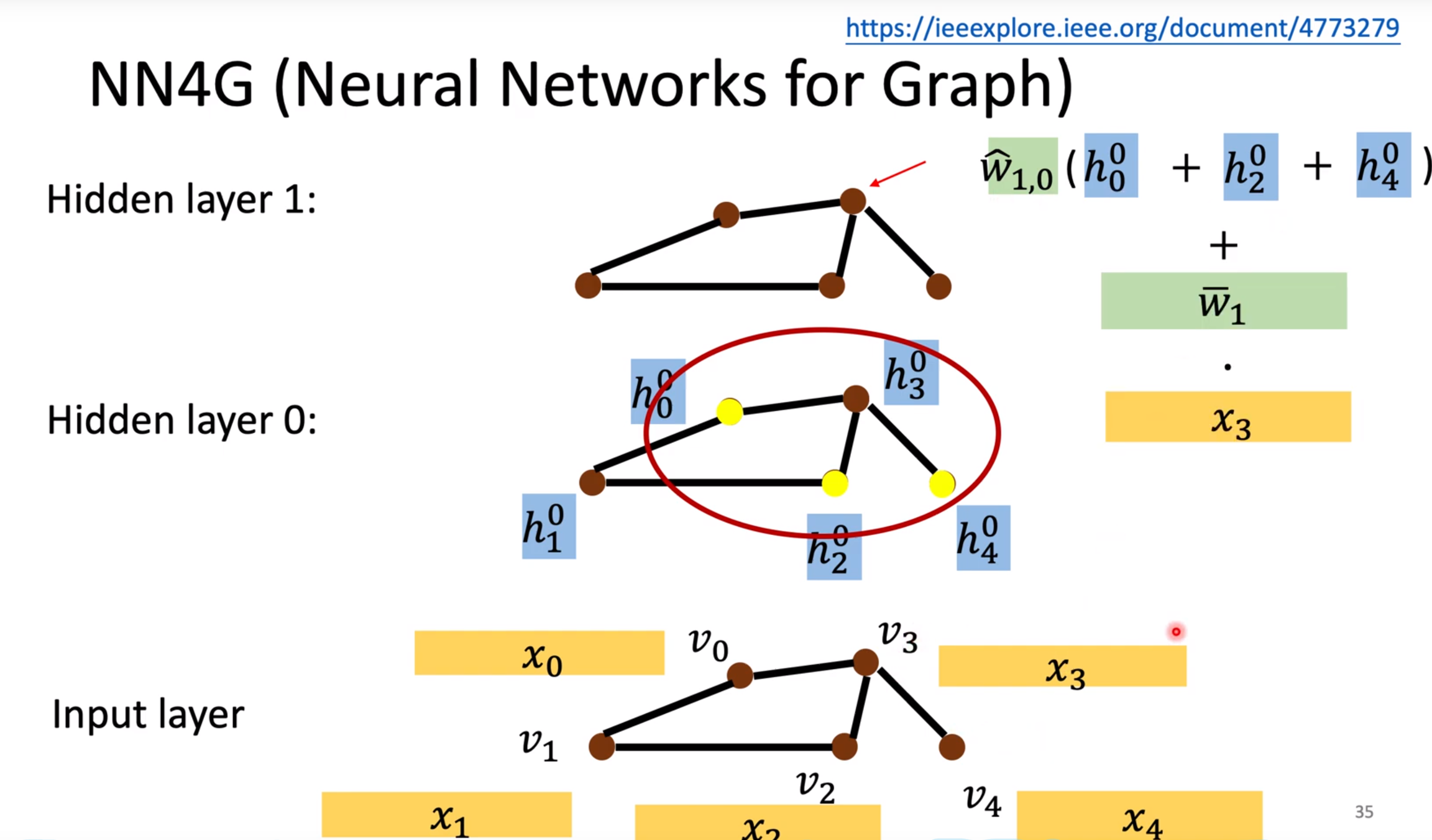
图神经网络基础 节点有节点的属性,边有边的属性
节点可以分为:labeled node和unlabeled node。
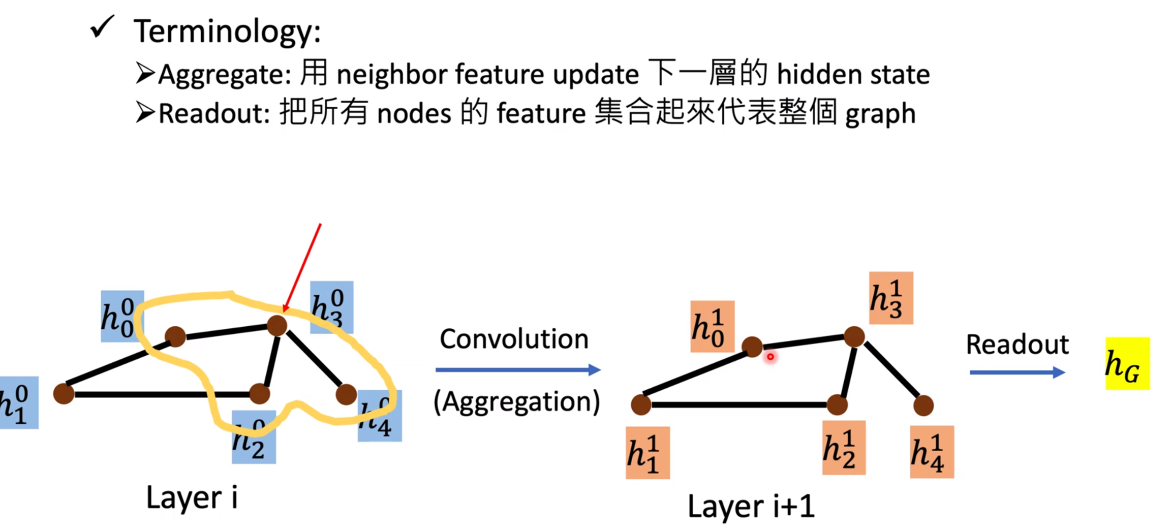
图卷积:
graph >> spatial-based convolution(空间卷积)
复制 15 15 # 作业数,机器数
6 94 12 66 4 10 7 53 3 26 2 15 10 65 11 82 8 10 14 27 9 93 13 92 5 96 0 70 1 83 # 奇数是机器索引,偶数是在该机器上的加工时间
4 74 5 31 7 88 14 51 13 57 8 78 11 8 9 7 6 91 10 79 0 18 3 51 12 18 1 99 2 33
1 4 8 82 9 40 12 86 6 50 11 54 13 21 5 6 0 54 2 68 7 82 10 20 4 39 3 35 14 68
5 73 2 23 9 30 6 30 10 53 0 94 13 58 4 93 7 32 14 91 11 30 8 56 12 27 1 92 3 9
7 78 8 23 6 21 10 60 4 36 9 29 2 95 14 99 12 79 5 76 1 93 13 42 11 52 0 42 3 96
5 29 3 61 12 88 13 70 11 16 4 31 14 65 7 83 2 78 1 26 10 50 0 87 9 62 6 14 8 30
12 18 3 75 7 20 8 4 14 91 6 68 1 19 11 54 4 85 5 73 2 43 10 24 0 37 13 87 9 66
11 32 5 52 0 9 7 49 12 61 13 35 14 99 1 62 2 6 8 62 4 7 3 80 9 3 6 57 10 7
10 85 11 30 6 96 14 91 0 13 1 87 2 82 5 83 12 78 4 56 8 85 7 8 9 66 13 88 3 15
6 5 11 59 9 30 2 60 8 41 0 17 13 66 3 89 10 78 7 88 1 69 12 45 14 82 4 6 5 13
4 90 7 27 13 1 0 8 5 91 12 80 6 89 8 49 14 32 10 28 3 90 1 93 11 6 9 35 2 73
2 47 14 43 0 75 12 8 6 51 10 3 7 84 5 34 8 28 9 60 13 69 1 45 3 67 11 58 4 87
5 65 8 62 10 97 2 20 3 31 6 33 9 33 0 77 13 50 4 80 1 48 11 90 12 75 7 96 14 44
8 28 14 21 4 51 13 75 5 17 6 89 9 59 1 56 12 63 7 18 11 17 10 30 3 16 2 7 0 35
10 57 8 16 12 42 6 34 4 37 1 26 13 68 14 73 11 5 0 8 7 12 3 87 2 83 9 20 5 97
复制 import pandas as pd
import numpy as np
from scipy.io import loadmat
复制 # AAS011R06.mat
m = loadmat('Data/P300/v2/AA001.mat')
m
复制 {'__header__': b'MATLAB 5.0 MAT-file, Platform: PCWIN, Created on: Thu Nov 29 14:36:17 2001',
'__version__': '1.0',
'__globals__': [],
'run': array([[3],
[3],
[3],
...,
[8],
[8],
[8]], dtype=uint8),
'trial': array([[ 0],
[ 0],
[ 0],
...,
[192],
[192],
[192]], dtype=uint8),
'sample': array([[ 0],
[ 1],
[ 2],
...,
[28829],
[28830],
[28831]], dtype=uint16),
'signal': array([[-1136, -416, -592, ..., -816, -496, -624],
[-1456, -912, -752, ..., -48, 336, -48],
[-1888, -912, -480, ..., -240, 0, 64],
...,
[-1952, -2416, -2336, ..., -1376, -2096, -1168],
[-2784, -2912, -2912, ..., 144, -800, -48],
[-1872, -1168, -1264, ..., 1008, 304, 816]], dtype=int16),
'TargetCode': array([[0],
[0],
[0],
...,
[0],
[0],
[0]], dtype=uint8),
'ResultCode': array([[0],
[0],
[0],
...,
[0],
[0],
[0]], dtype=uint8),
'StimulusTime': array([[51992],
[51992],
[51992],
...,
[54165],
[54165],
[54165]], dtype=uint16),
'Feedback': array([[0],
[0],
[0],
...,
[0],
[0],
[0]], dtype=uint8),
'IntertrialInterval': array([[1],
[1],
[1],
...,
[1],
[1],
[1]], dtype=uint8),
'Active': array([[1],
[1],
[1],
...,
[1],
[1],
[1]], dtype=uint8),
'SourceTime': array([[52082],
[52082],
[52082],
...,
[54256],
[54256],
[54256]], dtype=uint16),
'RunActive': array([[1],
[1],
[1],
...,
[1],
[1],
[1]], dtype=uint8),
'Recording': array([[1],
[1],
[1],
...,
[1],
[1],
[1]], dtype=uint8),
'IntCompute': array([[0],
[0],
[0],
...,
[0],
[0],
[0]], dtype=uint8),
'Running': array([[1],
[1],
[1],
...,
[1],
[1],
[1]], dtype=uint8)}
复制 for i in m:
try:
print(i,m[i].shape)
except:
continue
# 运行编号(runnr),运行内的强化次数(trinr)和运行内的样品编号(sample)
# 其他部分由于网页乱码看不出来,也可能说明文件中没有展示,需要浏览matlab文件
复制 run (172992, 1)
trial (172992, 1)
sample (172992, 1)
signal (172992, 64)
TargetCode (172992, 1)
ResultCode (172992, 1)
StimulusTime (172992, 1)
Feedback (172992, 1)
IntertrialInterval (172992, 1)
Active (172992, 1)
SourceTime (172992, 1)
RunActive (172992, 1)
Recording (172992, 1)
IntCompute (172992, 1)
Running (172992, 1) 每个字符:
矩阵显示时间2.5s,此时字符强度相等 ==> 视为空白
每一行和每一列被随机增强100ms,增强后,空白75ms
每次实验的单个通道信号量 = {2.5s + [(100+75) x 180 x 字符数]/1000 + 2.5s }x 240 Hz
台湾陈蕴侬视频2020 二、模型结构、损失函数、优化、反向传播
偏差(bias)的理解:相当于给一个初值,然后通过学习调整这个初值。
感知层(perception layer)的理解:每一层相当于一个切割,可以通过二层模拟出一个凸,越多层表达越多场景。
激活函数(activate function):选非线性的,线性跟权重没差。
损失函数(loss function):定义一个损失值,越小越接近正确的参数值。
梯度下降(Gradient Descent)的理解:越倾斜,下降越快,越平稳下降越慢;容易达到局部最小值,卡在局部。随机小批量梯度下降(SGD,选1个)比较快。小批量梯度下降(Mini-Batch GD,选k个).
训练速度:mini-batch>SGD>GD,因为现代电脑矩阵相乘的速度大于矩阵和向量相乘。
学习率:过大会学习过头,越过最小值。过小会学的很慢。
建议:1.数据随机;2.使用固定批量;3.调整学习率。
反向传播(backward propagation):通过梯度和学习率更新权重。其实就是微积分链式法则在模型中的体现。反向传播计算出的梯度乘以前向计算的结果,就是下一个变数的偏微分了。
共现矩阵:表示一起出现过的单词的关系。
奇异值分解(singular value decomposition,SVD):降低维度。
SVD问题:计算复杂度过高,难以加新词。
解决方法:降低维度,通过embedding的方法嵌入一个空间中的位置。常用word2vec,Glove方法。
知识型表示(knowledge-based representation):通过符号等来表示知识(知识图谱)
语料库表示(corpus-based representation):基于近邻的高维(共现矩阵),低维(降维或embedding);原子特征(atomic symbol,one-hot向量)
循环神经网络(recurrent neural net,RNN):将前面的影响传递给后面的网络。
梯度消失,梯度爆炸(Vanishing/Exploding Gradient):指数太多次,导致大的越大,小的越小。解决方法:裁剪(clipping)
双向循环神经网络(Bidirectional RNN):当时间可以双向的时候,可以使用。(不能预测股市这种单向时间的)
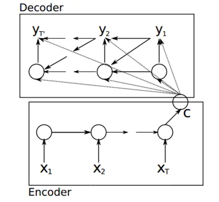
编码器-解码器:编码器生成W或背景向量C,解码器利用编码器结果来生成输出。
批量归一化计算:先归一化,后缩放和平移。
从经验法则来讲,L2正则化一般比L1正则化有效。
编码器-解码器实现注意力机制:编码器收集信息,收集完一整句(注意力在这)之后,保存在编码器,用解码器生成输出,直到遇到。
Q,K,V:Q是指query,K是指编码器中的key,V是指最后一层的Value。
最大化和最小化:多个概率相乘求其最大值,相当于对其求log后加个负号求最小值。也就是说,凡是求最大值的,都可以通过符号变成求最小值。
《第一章》 表示学习 ( Representation Learning):如果有一种算法可以自动地学习出有效的特征, 并提高最终机器学习模型的性能 .
局部表示 ( Local Representation):也叫离散表示,符号表示,例如one-hot向量。
分布式表示 ( Distributed Representation):例如RGB值,通常表示低维的稠密向量。
嵌入 (Embedding):使用神经网络,将高维的局部表示空间映射到非常低维的分布式表示空间,在这个低维的空间中,每个特征不再是坐标轴上的点,而是分散在整个低维空间中。自然语言中的分布式表示,也叫词嵌入 。
深度学习 (Deep Learning):为了学习一种好的表示, 需要构建具有一定“深度”的模型, 并通过学习算法来让模型自动学习出好的特征表示( 从底层特征, 到中层特征, 再到高层特征),从而最终提升预测模型的准确率. 所谓“深度” 是指原始数据进行非线性特征转换的次数 . 如果把一个表示学习系统看作是一个有向图结构, 深度也可以看作是从输入节点到输出节点所经过的最长路径的长度. 某种意义上可以看作一种强化学习(Reinforcement Learning)
深度学习采用的模型主要是神经网络模型 , 其主要原因是神经网络模型可以使用误差反向传播算法, 从而可以比较好地解决贡献度分配问题. 随着模型深度的不断增加, 其特征表示的能力也越来越强, 从而 使后续的预测更加容易
端到端学习 ( End-to-End Learning): 也称端到端训练, 是指在学习过程中不进行分模块或分阶段训练, 直接优化任务的总体目标. 在端到端学习中, 一般不需要明确地给出不同模块或阶段的功能, 中间过程不需要人为干预. 大部分采用神经网络模型的深度学习可以看作一种端到端的学习。
神经网络 (机器学习领域):由很多人工神经元构成的网络结构模型, 这些人工神经元之间的连接强度是可学习的参数.
赫布型学习 ( Hebbian learning):如果两个神经元总是相关联地受到刺激, 它们之间的突触强度增加.
凝固作用 :短期记忆转化为长期记忆的过程
网络容量 ( Network Capacity):指人工神经网络塑造复杂函数的能力, 与可以被储存在网络中的信息的复杂度以及数量相关
1.8总结
特征工程 :要开发一个实际的机器学习系统, 人们往往需要花费大量的精力去尝试设计不同的特征以及特征组合, 来提高最终的系统能力。
MXNet 主要是在20年暑假期间学习开源框架MXNet的开源书籍
《动手学习深度学习》:https://zh.d2l.ai/chapter_preface/preface.html
复制 torch.cuda.is_available()
复制 # 未初始化的矩阵
# 里面的值是不确定的
x = torch.empty(5,3)
print(x)
复制 # 构造随机初始化的矩阵
x = torch.rand(5,3)
x
复制 import torch
# 神经网络的包,仅支持小批量样本的训练,不支持单个样本(可以input.unsqueeze(0)来模拟批量[1])
import torch.nn as nn
import torch.nn.functional as F # 一些常用的函数
class Net(nn.Module):
def __init__(self):
super(Net, self).__init__()
self.conv1 = nn.Conv2d(1, 6, 3) # 卷积核
self.conv2 = nn.Conv2d(6, 16, 3) # 卷积核
# Linear是简单的映射函数,第一个参数w的维度,第二个参数b的维度
self.fc1 = nn.Linear(16 * 6 * 6, 120) # 6*6是图片的长宽
self.fc2 = nn.Linear(120, 84)
self.fc3 = nn.Linear(84, 10) # 最后输出10个分类
def forward(self, x):
x = F.max_pool2d(F.relu(self.conv1(x)), (2, 2)) # 最大二维池化层:2*2格子内取最大
x = F.max_pool2d(F.relu(self.conv2(x)), 2) # 第一个参数的结果是笔直的向量
x = x.view(-1, self.num_flat_features(x)) # -1表示自动计算,view是改变形状
x = F.relu(self.fc1(x))
x = F.relu(self.fc2(x))
x = self.fc3(x)
return x
def num_flat_features(self, x): # 每个输入变平后的数量大小
size = x.size()[1:] # 获得除了批量大小的所有维度
num_features = 1
for s in size:
num_features *= s
return num_features
net = Net()
print(net) # 获取当前模型的数据
复制 Net(
(conv1): Conv2d(1, 6, kernel_size=(3, 3), stride=(1, 1))
(conv2): Conv2d(6, 16, kernel_size=(3, 3), stride=(1, 1))
(fc1): Linear(in_features=576, out_features=120, bias=True)
(fc2): Linear(in_features=120, out_features=84, bias=True)
(fc3): Linear(in_features=84, out_features=10, bias=True)
)
复制 print(params[1]) # conv1的偏移
复制 tensor([[1.6880e+25, 2.5226e-18, 6.6645e-10],
[4.1575e+21, 1.3294e-08, 2.0773e+20],
[1.6536e-04, 1.0016e-11, 8.3391e-10],
[2.1029e+20, 2.0314e+20, 3.1369e+27],
[7.0800e+31, 3.1095e-18, 1.8590e+34]])
复制 tensor([[0.3129, 0.8714, 0.8079],
[0.4722, 0.3522, 0.3068],
[0.9920, 0.0171, 0.6463],
[0.1151, 0.7443, 0.1300],
[0.2816, 0.7904, 0.1833]])
复制 # 构造一个填充0,且数据类型dtype为long的矩阵
x = torch.zeros(5, 3, dtype=torch.long)
x
复制 tensor([[0, 0, 0],
[0, 0, 0],
[0, 0, 0],
[0, 0, 0],
[0, 0, 0]])
复制 # 将数组转换从tensor张量
x = torch.tensor([5.5, 3])
x
复制 tensor([5.5000, 3.0000])
复制 # 拷贝一个值
x = x.new_ones(5, 3, dtype=torch.double) # new_* methods take in sizes
print(x)
复制 tensor([[1., 1., 1.],
[1., 1., 1.],
[1., 1., 1.],
[1., 1., 1.],
[1., 1., 1.]], dtype=torch.float64)
复制 # 拷贝形状,并随机赋值-1到1之间
x = torch.randn_like(x, dtype=torch.float) # override dtype!
print(x) # result has the same size
复制 tensor([[0.1310, 0.8429, 0.9671],
[0.4961, 0.4118, 0.5708],
[0.9019, 0.1656, 0.9630],
[0.1138, 0.5194, 0.2060],
[0.0544, 0.8853, 0.4521]])
复制 # 拷贝形状,并随机赋值0到1之间
x = torch.rand_like(x, dtype=torch.float) # override dtype!
print(x) # result has the same size
复制 tensor([[0.2949, 0.5003, 0.8243],
[0.0197, 0.8175, 0.7986],
[0.2791, 0.1747, 0.9388],
[0.6410, 0.7757, 0.9517],
[0.5885, 0.8757, 0.0301]])
复制 # 获取矩阵大小
print(x.size())
复制 # 加法一,会生成新变量
y = torch.rand(5, 3)
print(x + y)
# 加法二,会生成新变量
print(torch.add(x, y))
复制 tensor([[0.8205, 1.1127, 0.9667],
[1.0123, 1.6212, 1.7500],
[0.7720, 0.5131, 1.8308],
[1.1216, 1.0681, 1.8199],
[1.4038, 1.3346, 0.7781]])
tensor([[0.8205, 1.1127, 0.9667],
[1.0123, 1.6212, 1.7500],
[0.7720, 0.5131, 1.8308],
[1.1216, 1.0681, 1.8199],
[1.4038, 1.3346, 0.7781]])
复制 # 加法三,设定指定的变量result为输出
result = torch.empty(5, 3)
torch.add(x, y, out=result)
print(result)
复制 tensor([[0.8205, 1.1127, 0.9667],
[1.0123, 1.6212, 1.7500],
[0.7720, 0.5131, 1.8308],
[1.1216, 1.0681, 1.8199],
[1.4038, 1.3346, 0.7781]])
复制 # 加法四:就地加法,不会生成新变量,但会改变其中一个参数
y.add_(x)
print(y)
复制 tensor([[0.8205, 1.1127, 0.9667],
[1.0123, 1.6212, 1.7500],
[0.7720, 0.5131, 1.8308],
[1.1216, 1.0681, 1.8199],
[1.4038, 1.3346, 0.7781]])
复制 tensor([[0.8205, 1.0123, 0.7720, 1.1216, 1.4038],
[1.1127, 1.6212, 0.5131, 1.0681, 1.3346],
[0.9667, 1.7500, 1.8308, 1.8199, 0.7781]])
复制 # 拷贝
x.copy_(y.t_())
# 任何使得张量发生变化的操作都需要添加下划线_
复制 tensor([[0.8205, 1.1127, 0.9667],
[1.0123, 1.6212, 1.7500],
[0.7720, 0.5131, 1.8308],
[1.1216, 1.0681, 1.8199],
[1.4038, 1.3346, 0.7781]])
复制 # 输出所有列,第1行
print(x[:, 1])
复制 tensor([1.1127, 1.6212, 0.5131, 1.0681, 1.3346])
复制 # 通过view改变形状
x = torch.randn(4, 4)
y = x.view(16)
z = x.view(-1, 8) # -1表示根据其他维度来推断
print(x.size(), y.size(), z.size())
复制 torch.Size([4, 4]) torch.Size([16]) torch.Size([2, 8])
复制 # 张量转化为数字
x = torch.randn(1)
print(x)
print(x.item())
复制 tensor([1.2919])
1.291871190071106
复制 # torch转NumPy
# 两个变量共享内存
a = torch.ones(5)
print(a)
b = a.numpy()
print(b)
a.add_(1)
print(a)
print(b)
复制 tensor([1., 1., 1., 1., 1.])
[1. 1. 1. 1. 1.]
tensor([2., 2., 2., 2., 2.])
[2. 2. 2. 2. 2.]
复制 # NumPy转torch
# 自动转化
import numpy as np
a = np.ones(5)
b = torch.from_numpy(a)
np.add(a, 1, out=a)
print(a)
print(b)
# CharTensor不支持转化为NumPy
复制 [2. 2. 2. 2. 2.]
tensor([2., 2., 2., 2., 2.], dtype=torch.float64)
复制 # 以下代码只有在PyTorch GPU版本上才会执行
if torch.cuda.is_available():
device = torch.device("cuda") # GPU
y = torch.ones_like(x, device=device) # 直接创建一个在GPU上的Tensor
x = x.to(device) # 改变环境,等价于 .to("cuda")
z = x + y
print(z)
print(z.to("cpu", torch.double)) # to()还可以同时更改数据类型
复制 tensor([1.1416, 2.4353], device='cuda:0')
tensor([1.1416, 2.4353], dtype=torch.float64)
复制 tensor([1., 1.], device='cuda:0')
复制 params = list(net.parameters())
print(len(params)) # 自动学习参数的数量
print(params[0].size()) # 6*1*3*3 ,conv1的权重
复制 10
torch.Size([6, 1, 3, 3])
复制 Parameter containing:
tensor([ 0.0176, 0.2514, 0.1497, 0.1647, -0.2829, 0.0409],
requires_grad=True)
复制 input = torch.randn(1,1,32,32)
out = net(input)
print(out) # 输出,数值最大的是正确分类,但一开始没有训练是随机的
复制 tensor([[ 6.9398e-03, -6.6113e-05, -6.9214e-02, -7.6395e-02, 3.9166e-02,
-7.0978e-02, 1.2993e-02, -1.7690e-02, -1.4292e-02, -4.7204e-02]],
grad_fn=<AddmmBackward>)
复制 net.zero_grad() # 设置所有梯度为0
out.backward(torch.randn(1,10)) # 设置随机数为梯度
复制 output = net(input)
target = torch.randn(10) # 假设一个假的结果
target = target.view(1, -1) # 变为[1,10]形状
criterion = nn.MSELoss() # 均方误差
loss = criterion(output, target)
print(loss)
复制 tensor(0.7828, grad_fn=<MseLossBackward>)
复制 """
input -> conv2d -> relu -> maxpool2d -> conv2d -> relu -> maxpool2d
-> view -> linear -> relu -> linear -> relu(3) -> linear(2)
-> MSELoss(1)
-> loss
"""
print(loss.grad_fn) # MSELoss
print(loss.grad_fn.next_functions[0][0]) # Linear
print(loss.grad_fn.next_functions[0][0].next_functions[0][0]) # ReLU
复制 <MseLossBackward object at 0x7fefaac1c8d0>
<AddmmBackward object at 0x7fefaac1ca90>
<AccumulateGrad object at 0x7fefaac1c8d0>
复制 net.zero_grad()
print('conv1.bias.grad before backward') # 反向传播之前
print(net.conv1.bias.grad)
loss.backward()
print('conv1.bias.grad after backward') # 反向传播后
print(net.conv1.bias.grad)
复制 conv1.bias.grad before backward
tensor([0., 0., 0., 0., 0., 0.])
conv1.bias.grad after backward
tensor([-0.0158, -0.0015, -0.0017, 0.0073, 0.0074, -0.0123])
复制 # 更新权重
learning_rate = 0.01
for f in net.parameters():
f.data.sub_(f.grad.data * learning_rate) # sub_是减等于
复制 import torch.optim as optim # 优化算法包
optimizer = optim.SGD(net.parameters(), lr=0.01) # 创建优化算法器
optimizer.zero_grad() # 初始化梯度为0
output = net(input) # 前向传播
loss = criterion(output, target) # 计算损失
loss.backward() # 反向传播
optimizer.step() # 更新权重 感知伴侣满意度
依恋回避
这些变量并没有增加信息,都无法预测谁的关系质量会随着时间的推移而增加或减少
选择最好的预测器 构建决策树,并在未使用的数据上测试预测能力
分别产生了数千个决策树,然后使用平均值结合在一起。
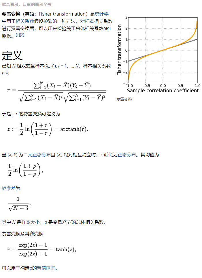
为了计算每个效应量,我们将随机森林模型结果的“方差占比”转换为效应大小r(通过取平方根) ;
不纯度(impurity)在分类中通常为Gini不纯度或信息增益/信息熵,对于回归问题来说是方差。
概率越大,纯度(或熵)越小 ,即发生的不确定性越小
然后我们进行Fisher-zr变换,我们使用N-3作为逆方差权重,其中N等于随机森林中使用的观察数分析
z' = 0.5 * ln((1+z)/(1-z))
我们将meta分析的结果转换回结果中占百分比的方差(通过将值平方 )
阅读全文后再剔除,2篇重复,2篇不是手稿,1篇没有临床,3篇质量差
2项包括贝叶斯置信网络 和动态时间扭曲(DTW) 算法
早期检测可以及时修正风险因素达到高质量的HD实验和有利的结果
诊断
用人工智能评估动静脉瘘管的流通性可以改善HD实验的结果和病人的生命质量
通过用人工智能解决方案代替更昂贵的诊断流程能减少医疗成本
处方
人工智能推荐药物剂量预防HD相关的并发症如贫血和血红蛋白的波动、矿物质失衡等
算法的参与会导致更少的并发症和减少药物的使用,减少治疗费用
预测
特定的算法预测生命质量,对心血管的测量结果和透析内的血流动力学事件的变化
生存和生命质量预测模型可以减轻对公共卫生的影响,更好的指导资源的使用
预测血流动力学事件通过避免低血压、心率和容量的变异性以实时适应HD过程,从而保证HD实验的成功和整体成本效益的干预措施。
挑战和需要更多人工智能研究的HD领域
实时监控的人工智能系统通过在HD实验中的嵌入式自动适应性反应以实现个性化治疗
通过AI/ML系统和专家负责的HD实验的反馈实现两者之间潜在的相互作用,使得两个部分相互学习,为ESRD患者提供更好的决策。
更多的人工智能系统将部署在HD病人护理上,这会产生规模更大的数据。应促使制定有关数据隐私、维护和共享的严格法规,以便在公共医疗保健中更安全地实施
实验三
结合生物标记测量期间急性腹膜炎和基于支持向量机、神经网络和随机森林的特征选择方法,一项研究(包括83 PD患者腹膜炎)证实了先进的数学模型在分析复杂的生物医学数据集和强调感染部位病原体特异性炎症反应的关键途径方面的强大作用。
实验四
利用CAPD患者的数据挖掘模型,提取模式,根据他们的血液分析对卒中风险患者进行分类。在最近的一项研究中,分析了850个病例的数据集,五种不同的人工智能算法(朴素贝叶斯、逻辑回归、MLP、随机森林和k-NN)被用来预测患者的中风风险。RT和k-NN预测脑卒中风险的特异性和敏感性均为95%。
人工智能算法可以发现生物标志物特征与不同类型的感染之间的联系
对早期采取适当的治疗方法以及避免易感ESRD患者的严重感染并发症有巨大的意义
AI通过突出PD中病原体特异性炎症反应所涉及的关键途径,为扩大病理生理机制的科学知识做出贡献
处方
通过使用人工智能,将透析前患者分为高转运蛋白组和低转运蛋白组,可以为尿毒症患者提供更好的治疗选择,这将改善PD患者的预后(根据经验预测的疾病发展情况),降低发病率和死亡率
预测
算法可以识别患者中风的风险,因此允许早期干预和减少PD的住院数
挑战和需要更多人工智能研究的PD领域
人工智能可以用来识别有腹膜炎风险的患者,以降低感染风险,克服腹膜透析过程中的巨大负担
在自动化PD中开展家庭远程监测的研究可以改善患者的治疗结果和对治疗的坚持
对使用吸附剂技术的透析液再生制造自动化可穿戴人工肾PD装置的安全性的研究
实验三
DTW(动态时间规整算法)用于识别一系列实验室数据中的异常模式,从而早期发现并报告与急性排斥反应相关的肌酐病程[56]。对数据库中存储的1,059,403个实验室值、43,638个肌酐测量值、1143名患者和680次排斥事件进行数据提取。通过将人工智能集成到电子患者登记系统中,可以前瞻性地评估对移植受者护理的真正影响。
实验四
在一项对257名接受KT的儿科患者进行的回顾性研究中,采用了一个经过反向传播训练的MLP,使用20个简单的输入变量来确定血清肌酐的延迟下降(移植肾功能恢复的延迟)[57]。据报道,其他模型(决策树)突出了有移植物丢失风险的受试者。
实验五
使用USRDS数据库中的数据集(来自5144名患者的48个临床变量),开发了一个作为移植前器官匹配工具的M1软件(基于贝叶斯信念网络(BBN))。该模型可以预测第一年内移植失败,特异性为80%。
实验六
对1045名KT患者进行研究,8项ML技术接受了基于药物遗传算法的TSD()预测培训。确定了与TSD显著相关的临床和遗传因素。高血压、奥美拉唑的使用和CYP3A5基因型用于构建多元线性回归(MLR)
实验七
一项涉及129名KT患者的前瞻性研究证实,通过神经网络将多个ABCB1多态性与CYP3A5基因型结合起来,可以更准确地计算出他克莫司的初始剂量,从而改善治疗并预防他克莫司毒性。
实验八
37名KT患者被随机分为低脂标准组和地中海饮食组。对于黄斑变性组,神经网络有两个隐藏层,分别有223个和2个神经元。在对照组中,网络也有两个隐藏层,分别有148个和2个神经元。结论是在不影响血脂水平的情况下,地中海饮食对移植后患者是理想的。该报告是唯一一项评估移植后不同类型饮食优势的研究。
处方
各种ML模型准确地预测他克莫司稳定的剂量,成功改善移植后的免疫抑制治疗和预防他克莫司毒性
ML可以评估移植手术后不同类型的饮食的优势,可以使KT对生命质量产生积极的影响
预测
人工智能被用于预测移植排斥反应、“移植延迟功能”和死亡率
人工智能算法可做作为移植前器官匹配工具,使得器官的分配更加合理,从整体优化KT医疗保健管理系统
挑战和需要更多人工智能研究的KT领域
预防性的人工智能工具可以用于识别移植物排斥和移植物丢失的可变危险因素,为病人提供成功率更高的KT
指导方针需要支持使用人工智能来分配器官或预测排斥反应
通过将人工智能整合到电子病人登记系统中,可以很容易地对人工智能对移植受者护理的影响进行前瞻性评估
我们期望在未来几年,所有肾移植程序将通过人工智能管理
透析服务管理,透析程序,贫血管理,激素/饮食问题,动静脉瘘(异常通道)评估
管理系统(ML用作移植前器官匹配工具),预测移植排斥反应,他克莫斯(肝肾移植的一线用药)治疗调节,饮食问题
透析服务管理,透析程序,贫血管理,激素/饮食问题,动静脉瘘(异常通道)评估
管理系统(ML用作移植前器官匹配工具),预测移植排斥反应,他克莫斯(肝肾移植的一线用药)治疗调节,饮食
Random walks
Graph auto encoders (GAE)
第一想法:传统自编码器,用隐藏向量还原原始数据,即训练目标为output拟合原始数据
进一步想法:变分自编码器,为每个样本构造专属的正态分布,然后采样获得隐藏向量来重构。隐藏向量的分布尽量能接近高斯分布,能够随机生成隐含变量喂给解码器,也提高了泛化能力。
但是,对于数据集和任务来说,完成任务所需要的特征并不一定要能完成图像重构。例如,辨别百元假钞不一定要能完整复刻出百元假钞。
互信息(MI, mutual information)
好特征的基本原则应当是**“能够从整个数据集中辨别出该样本出来”**,也就是说,提取出该样本(最)独特 的信息。
熵H(Y)与条件熵H(Y|X)之差称为互信息,决策树学习中的信息增益等价于训练数据集中类与特征的互信息。
互信息:变量间相互依赖性 的量度。不同于相关系数,互信息并不局限于实值随机变量。它能度量两个事件集合之间的相关性。
用 X 表示原始图像的集合,用 x∈X 表示某一原始图像。
Z 表示编码向量的集合,z∈Z 表示某个编码向量。
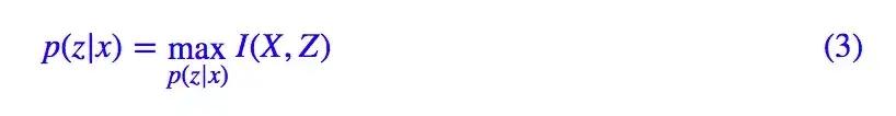
p(z|x) 表示 x 所产生的编码向量的分布,我们设它为高斯分布。这是我们要找的编码器 。
p̃(x) 原始数据的分布,p(z) 是在 p(z|x) 给定之后整个 Z 的分布
I(X, Z) = H(Z) - H(Z|X) :熵 H(Z) 看作一个随机变量不确定度的量度,那么 H(Z|X) 就是 X 没有涉及到的 Z 的部分的不确定度的量度。总的Z的不确定度,减去知道X而剩下的Y的不确定度,所以可以直观地理解互信息是Z变量提供给Y的信息量
增强机制:对图的结构进行增广,然后对相同的节点进行子采样。类似于CV中的裁剪。
两个专用的GNN:即图编码器。对应原数据和增强后的数据。
使用GCN。σ(AXΘ) and σ(SXΘ), X为初始节点的特征,Θ为学习参数。
一个共享的MLP(靠左):用于学习图的节点表示 。具有两个隐藏层和PReLU激活函数。
一个图池化层P:即readout函数,而后传入共享MLP(结构同上)中,得出图表示 。
每个GCN层中的节点表示的总和,连接起来,然后将它们馈送到一个单层前馈网络。
鉴别器D:图的节点表示 和另一个图的图形表示 进行对比。并对它们的一致性进行评分。
Θ是权重系数,表示全局和局部信息的比例。所有θ之和为1。
heat kernel : 带入T = AD-1, θk = α(1-α)k。α是随机游走的传送概率,t是
Personalized PageRank : 带入T = D-1/2AD-1/2, θk = e-ttk/k!
从一个图中随机采样节点及边,然后再从另一个图(扩散后)中确定对应的节点和边。
扩充view的数量超过两个不会改善性能,最好的效果是邻接矩阵和传播矩阵 进行对比学习。
对比节点和视图的表示 达到更好的效果,优于,图-图表示对比学习,不同长度的编码对比学习。
**简单的图读出层(求和)**比differentiable pooling(DiffPool)效果更好。
预训练时候,应用正则化(提前停止除外)或规范化层会对性能产生负面影响。
Tensor
,去翻翻官方API就知道了,下表给了一些常用的作参考。
这些创建方法都可以在创建的时候指定数据类型dtype和存放device(cpu/gpu)。
另外,PyTorch还支持一些线性函数,这里提一下,免得用起来的时候自己造轮子,具体用法参考官方文档。如下表所示:
addmm/addbmm/addmv/addr/baddbmm..
当对两个形状不同的Tensor按元素运算时,可能会触发广播(broadcasting)机制:先适当复制元素使这两个Tensor形状相同后再按元素运算。
所有在CPU上的Tensor(除了CharTensor)都支持与NumPy数组相互转换。
Tensor是这个包的核心类,如果将其属性.requires_grad设置为True,它将开始追踪(track)在其上的所有操作(这样就可以利用链式法则进行梯度传播了)。完成计算后,可以调用.backward()来完成所有梯度计算。此Tensor的梯度将累积到.grad属性中。
注意在y.backward()时,如果y是标量,则不需要为backward()传入任何参数;否则,需要传入一个与y同形的Tensor。解释见 2.3.2 节。
如果不想要被继续追踪,可以调用.detach()将其从追踪记录中分离出来,这样就可以防止将来的计算被追踪,这样梯度就传不过去了。
可以用with torch.no_grad()将不想被追踪的操作代码块包裹起来,这种方法在评估模型的时候很常用,因为在评估模型时,我们并不需要计算可训练参数(requires_grad=True)的梯度。
Function是另外一个很重要的类。Tensor和Function互相结合就可以构建一个记录有整个计算过程的有向无环图(DAG)。
每个Tensor都有一个.grad_fn属性,该属性即创建该Tensor的Function, 就是说该Tensor是不是通过某些运算得到的,若是,则grad_fn返回一个与这些运算相关的对象,否则是None。
tensor.requires_grad 用于说明当前量是否需要在计算中保留对应的梯度信息
标量out,直接调用out.backward();不允许使用张量对张量求导,需要加权平均,例如out.backward(w);
如果我们想要修改tensor的数值,但是又不希望被autograd记录(即不会影响反向传播),那么我么可以对tensor.data进行操作。
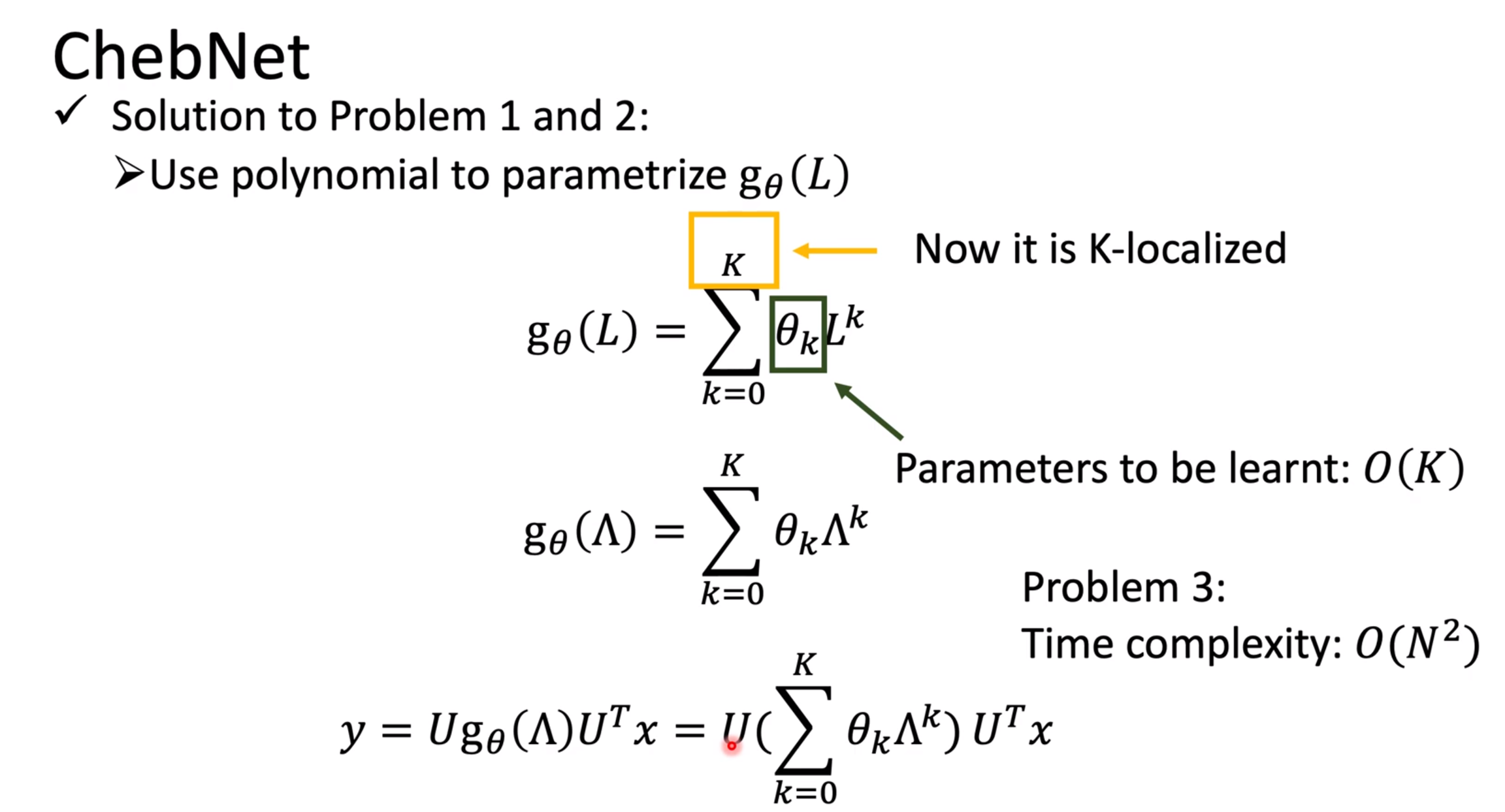
Fourier Domain(傅里叶变化) ; Spectral-based convolution
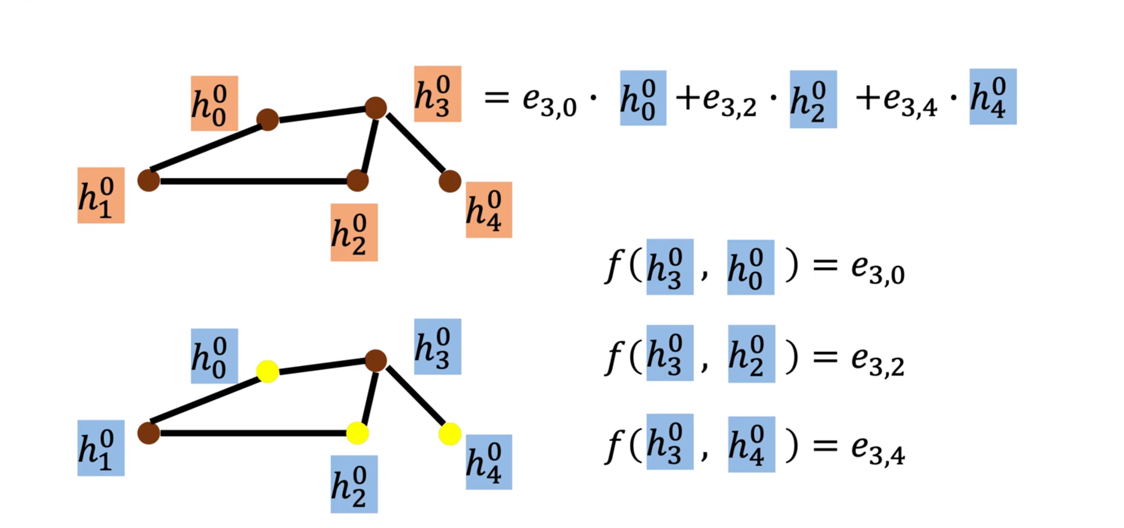
重点:GAT(graph attention network),GCN
L是半正定,特征值都是大于等于0。Lf中的第i个结果代表了第i点和相邻节点的差。
fTLf代表了两个点的能量差异,可以当作一种“能量”,“频率”来使用。
复制 import torch
import torchvision # 常用数据集包
import torchvision.transforms as transforms # 数据转归一化
复制 transform = transforms.Compose( # 自定义一个转换器,先变成张量,再归一化(每个通道的均值序列,标准差序列)
[transforms.ToTensor(),
transforms.Normalize((0.5, 0.5, 0.5), (0.5, 0.5, 0.5))]) # (0-0.5)/0.5 = -1
trainset = torchvision.datasets.CIFAR10(root='./data', train=True, download=True,
transform=transform)
trainloader = torch.utils.data.DataLoader(trainset, batch_size=4, shuffle=True,
num_workers=2)
testset = torchvision.datasets.CIFAR10(root='./data', train=False, download=True,
transform=transform)
testloader = torch.utils.data.DataLoader(testset, batch_size=4, shuffle=False,
num_workers=2)
# num_workers根据计算机的CPU和内存来设置,充足可以设置多一些
# 设为0表示不用内存
classes = ('plane','car', 'bird','cat','deer', 'dog','frog','horse','ship','truck')
复制 Files already downloaded and verified
Files already downloaded and verified
《第四章》 定义:构成神经网络的基本单元,其主要是模拟生物神经元的结构和特性,接收一组输入信号并产出 输出 激活函数特定: (1)连续并可导(允许少数点上不可导)的非线性函数. 可导的激活函数可以直接利用数值优化 的方法来学习网络参数.
(2) 激活函数及其导函数要尽可能的简单 ,有利于提高网络计算效率.
(3) 激活函数的导函数的值域要在一个合适的区间 内, 不能太大也不能太小,否则会影响训练的效率和稳定性.
4.1.1 Sigmoid函数
Sigmoid型函数是指一类 S型曲线函数,为两端饱和函数. (𝑥 → −∞时,其导数 𝑓′(𝑥) → 0,则称其为左饱和)
常用的 Sigmoid型函数: Logistic函数 和 Tanh函数 .
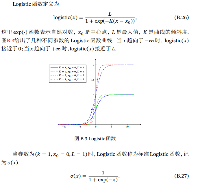
Logistic: 𝜎(𝑥) = 1/[1 + exp(−𝑥)]理解:把一个实数域的输入“ 挤压” 到(0, 1). 当输入值在 0附近时,Sigmoid型函数近似为线性函数;当输入值靠近两端时,对输入进行抑制. 输入越小,越接近于 0;输入越大,越接近于 1. 特征: - 其输出直接可以看作是概率分布 - 其可以看作是一个软性门(Soft Gate),用来控制其他神经元输出信息的数量tanh(𝑥) = (exp(𝑥) − exp(−𝑥))/(exp(𝑥) + exp(−𝑥))tanh(𝑥) = 2𝜎(2𝑥) − 1
理解:看作是放大并平移的 Logistic函数,其值域是(−1,1)
4.1.1.1 Hard-Logistic函数和 Hard-Tanh函数
两个函数:
ReLU(Rectified Linear Unit,修正线性单元)
ReLU(𝑥) = max(0,𝑥)理解: ReLU 却具有很好的稀疏性, 大约50% 的神经元会处于激活状态.被认为有生物上的解释性,比如单侧抑制、宽兴奋边界(即兴奋程度也可以非常高). ReLU 函数为左饱和函数,且在𝑥 > 0时导数为 1,在一定程度上缓解了神经网络的梯度消失问题,加速梯度下降的收敛速度
缺点:死亡 ReLU 问题(Dying ReLU Problem),如果参数在一次不恰当的更新后,第一个隐藏层中的某个 ReLU神经元在所有的训练数据上都不能被激活, 那么这个神经元自身参数的梯度永远都会是 0,在以后的训练过程中永远不能被激活.
4.1.2.1 带泄漏的ReLU
LeakyReLU(𝑥) = max(0,𝑥) + 𝛾 min(0,𝑥)当𝛾 < 1时:LeakyReLU(𝑥) = max(𝑥,𝛾𝑥)
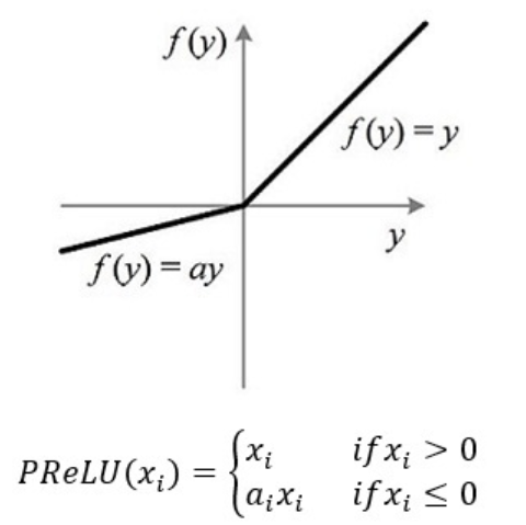
4.1.2.2 带参数的ReLU
PReLU𝑖(𝑥)= max(0, 𝑥) + 𝛾_𝑖 min(0, 𝑥)
𝛾_𝑖 为 𝑥 ≤ 0 时函数的斜率. 因此, PReLU 是非饱和函数. 如果 𝛾𝑖 = 0, 那么PReLU就退化为 ReLU. 如果 𝛾𝑖 为一个很小的常数,则 PReLU可以看作带泄露的ReLU. PReLU 可以允许不同神经元具有不同的参数 ,也可以一组神经元共享一个参数.
ELU(x) = = max(0, 𝑥) + min(0, 𝛾(exp(𝑥) − 1))
𝛾 ≥ 0是一个超参数,决定 𝑥 ≤ 0时的饱和曲线,并调整输出均值在 0附近
4.1.2.4 Softplus函数
Softplus(𝑥) = log(1 + exp(𝑥))
看作是 Rectifier 函数的平滑版本,其导数刚好是 Logistic函数. Softplus函数虽然也具有单侧抑制、宽兴奋边界的特性,却没有稀疏激活性.
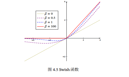
swish(𝑥) = 𝑥𝜎(𝛽𝑥)𝜎(⋅) 为 Logistic 函数, 𝛽 为可学习的参数或一个固定超参数. 𝜎(⋅)∈ (0, 1) 可以看作是一种软性的门控机制. 接近1为开,接近0为关.
当 𝛽 = 0时,Swish函数变成线性函数 𝑥/2.
当 𝛽 = 1时,Swish函数在 𝑥 > 0时近似线性, 在 𝑥 < 0 时近似饱和,同时具有一定的非单调性.
当 𝛽 → +∞ 时,𝜎(𝛽𝑥)趋向于离散的 0-1函数,Swish函数近似为 ReLU函数.
Swish函数可以看作是线性函数和 ReLU函数之间的非线性插值函数,其程度由参数 𝛽 控制
高斯误差线性单元(Gaussian Error Linear Unit,GELU),类似swish,用门控机制来调整输出值
GELU(𝑥) = 𝑥𝑃(𝑋 ≤ 𝑥)𝑃(𝑋 ≤ 𝑥)是高斯分布𝒩(𝜇,𝜎2)的累积分布函数,𝜇,𝜎为超参数,一般设 𝜇 = 0,𝜎 = 1即可.
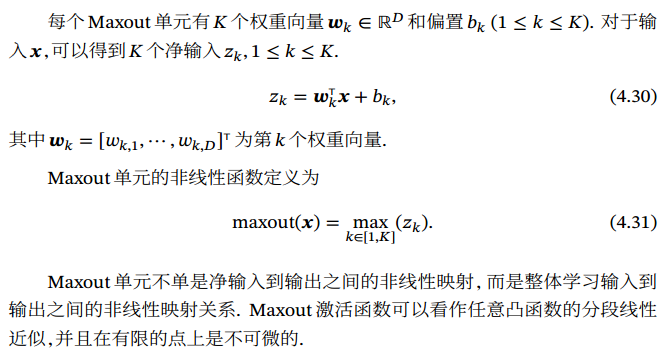
Maxout单元是一种分段线性函数.
Sigmoid 型函数、ReLU等激活函数的输入是神经元的净输入𝑧,是一个标量 .
Maxout单元的输入是上一层神经元的全部原始输出,是一个向量 𝒙 = [𝑥1;𝑥2;⋯;𝑥𝐷].
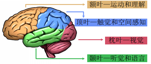
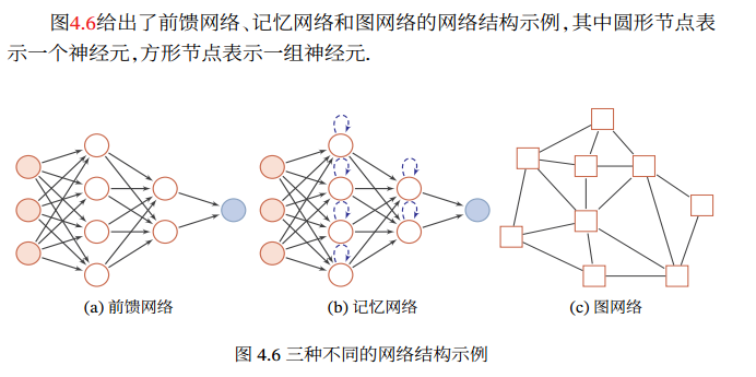
神经网络 :通过一定的连接方式或信息传递方式进行协作的神经元.
整个网络中的信息是朝一个方向传播,没有反向 的信息传播,可以用一个有向无环路图 表示.
前馈网络包括全连接前馈网络 和卷积神经网络 等.
前馈网络可看作一个函数,通过简单非线性函数的多次复合,实现输入空间到输出空间的复杂映射
记忆网络,也称为反馈网络 ,网络中的神经元不但可以接收其他神经元的信 息, 也可以接收自己的历史信息. 在不同的时刻具有不同的状态.
记忆神经网络中的信息传播可以是单向或双向传递,因此可用一个有向循环图或无向图 来表示. 为了增强记忆网络的记忆容量,可以引入外部记忆单元和读写机制,用来保存一些网络的中间状态, 称为记忆增强神经网络(Memory Augmented Neural Network,MANN)(第8.5节),比如神经图灵机和记忆网络记忆网络包括循环神经网络(第6章)、Hopfield网络(第8.6.1节)、玻尔兹曼机(第12.1节)、受限玻尔兹曼机(第12.2节)等.
记忆网络可以看作一个程序,具有更强的计算和记忆能力
实际应用中很多数据是图结构的数据,比如知识图谱、社交网络、分子(Molecular )网络等.
图网络是定义在图结构数据上的神经网络
图网络是前馈网络和记忆网络的泛化,包含很多不同的实现方式,比如图卷 积网络(Graph Convolutional Network, GCN)[Kipf et al., 2016]、 图注意力网络(Graph Attention Network,GAT)[Veličković et al., 2017]、消息传递神经网络(Message Passing Neural Network,MPNN)[Gilmer et al., 2017]等.
前馈神经网络(Feedforward Neural Network,FNN):多层的 Logistic回归模型(连续的非线性函数)组成.
第 0层称为输入层,最后一层称为输出层,其他中间层称为隐藏层.
第l-1层活性值(Activation):𝒂(𝑙−1)
第l层神经元的净活性值(Net Activation)𝒛(𝑙)
多层感知器(Multi-Layer Perceptron, MLP):由多层的感知器(不连续的非线性函数)组成.
通用近似定理 (Universal approximation theorem,一译万能逼近定理)」:如果一个前馈神经网络具有线性输出层和至少一层隐藏层,只要给予网络足够数量的神经元,便可以实现以足够高精度来逼近任意一个在 ℝn 的紧子集 (Compact subset) 上的连续函数。
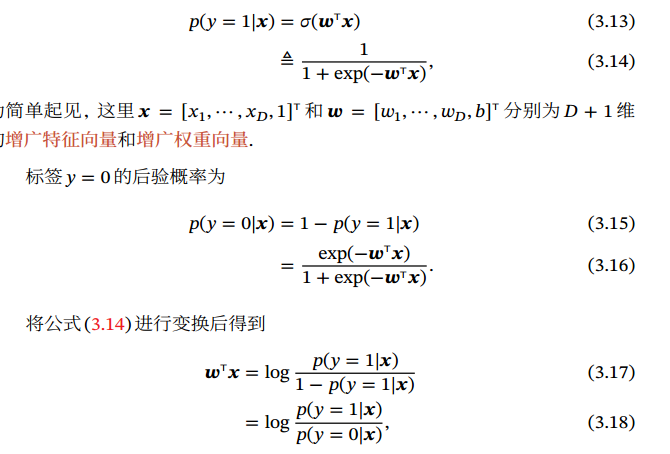
对于二分类问题𝑦 ∈ {0,1}, 并采用 Logistic 回归, 那么 Logistic 回归分类器可以看成神经网络的最后一层. 也就是说,网络的最后一层只用一个神经元,并且激活函数为 Logistic函数. 网络的输出可以直接作为类别𝑦 = 1的后验概率.
𝑝(𝑦 = 1|𝒙) = 𝑎(𝐿),
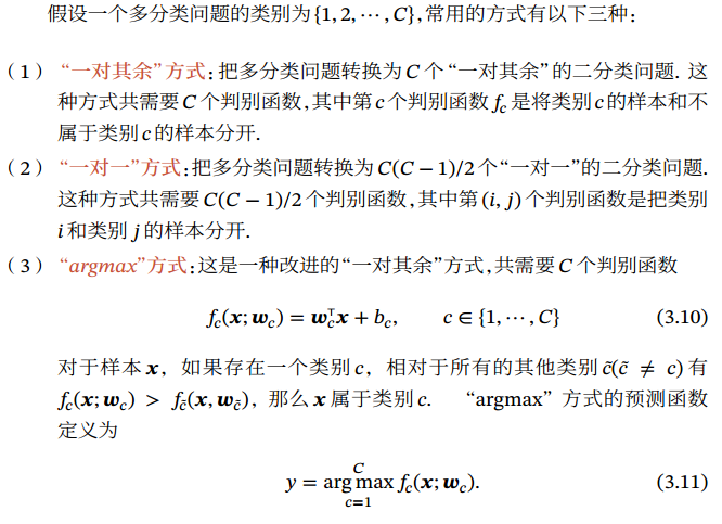
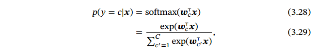
对于多分类问题,如果使用 Softmax 回归分类器,相当于网络最后一层设置𝐶 个神经元,其激活函数为 Softmax函数. 网络最后一层(第𝐿层)的输出可以作为每个类的后验概率.
̂y = softmax(𝒛(𝐿))
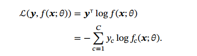
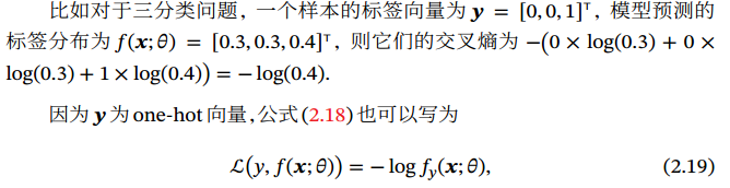
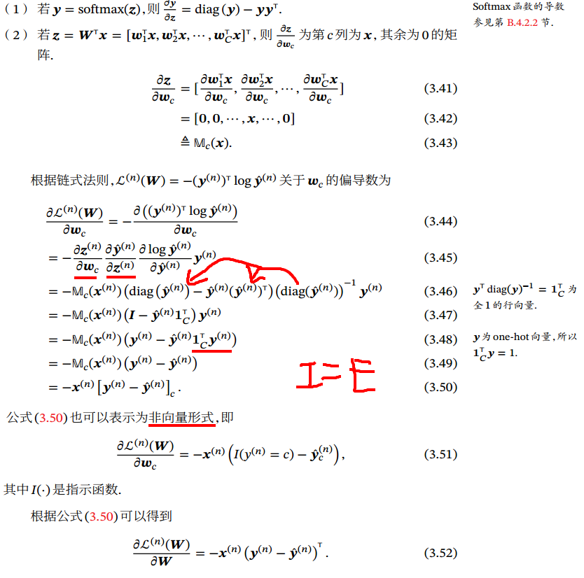
交叉熵损失函数:ℒ(𝒚,𝒚) = − ̂y^T log(𝒚).𝒚 ∈ {0,1}^𝐶 为标签𝑦 对应的 one-hot向量表示.
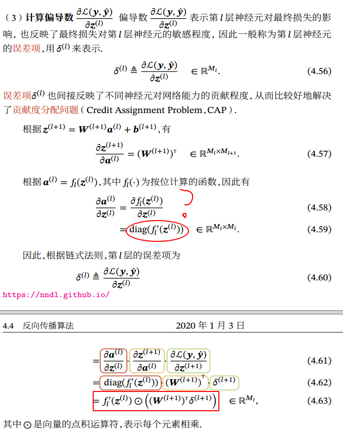
矩阵积分分三种形式: 反向传播算法 的含义是:第𝑙 层的一个神经元的误差项(或敏感性)是所有与该神经元相连的第 𝑙 + 1层的神经元的误差项的权重和. 然后,再乘上该神经元激活函数的梯度.
使用误差反向传播算法的前馈神经网络训练过程可以分为以下三步:
前馈计算每一层的净输入 𝒛(𝑙) 和激活值 𝒂(𝑙),直到最后一层;
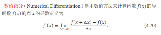
过小,会引起数值计算问题,比如舍入误差(Round-off Error)近似值和精确值的差异;
过大,会增加截断误差(Truncation Error)是指理论解和精确解之间的误差.
一种基于符号计算的自动求导方法.符号计算也叫代数计算. 例如x^2的导数是2x
缺点:
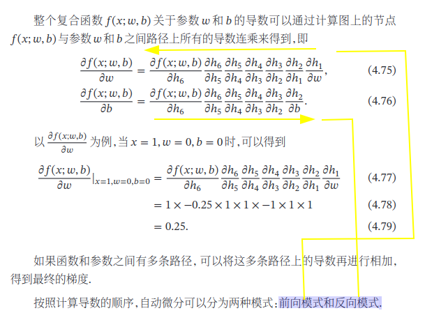
4.5.3 自动微分(Automatic Differentiation, AD)
自动微分的处理对象是一个函数或一段程序. 所有的数值计算可以分解为一些基本操作,然后利用链式法则 来自动计算一个复合函数的梯度.
前向模式需要对每一个输入变量都进行一遍遍历,共需要𝑁遍.
反向模式需要对每一个输出都进行一个遍历,共需要𝑀遍.
风险函数为𝑓 ∶ ℝ^𝑁→ ℝ,输出为标量,因此采用反向模式为最有效的计算方式,只需要一遍计算
静态计算图 是在编译时构建计算图,计算图构建好之后在程序运行时不能改变,静态计算图在构建时可以进行优化,并行能力强,但灵活性比较差.
动态计算图 是在程序运行时动态构建.两种构建方式各有优缺点.动态计算图则不容易优化,当不同输入的网络结构不一致时,难以并行计算,但是灵活性比较高.
Theano和Tensorflow1.x采用的是静态计算图,Tensorflow 2.0也支持了动态计算图.而DyNet、Chainer和PyTorch采用的是动态计算
神经网络的优化问题是一个非凸优化问题.(局部最小值不是全局最小值)
Logistic函数导数 :𝜎′(𝑥) = 𝜎(𝑥)(1 − 𝜎(𝑥))∈ [0,0.25]
Tanh函数导数 :tanh′(𝑥) = 1 −(tanh(𝑥))^2 ∈ [0,1]
梯度消失问题(Vanishing Gradient Problem):当网络层数增多时,梯度会不断衰减,直至消失.
解决方法:
《第一章》《第二章》 研究如何使计算机系统利用经验改善性能。
关注如何自动找出表示数据的合适方式,以便更好地将输入变换为正确的输出。
具有多级表示的表征学习方法。在每一级(从原始数据开始),深度学习通过简单的函数将该级的表示变换为更高级的表示。因此,深度学习模型也可以看作是由许多简单函数复合而成的函数。当这些复合的函数足够多时,深度学习模型就可以表达非常复杂的变换。
端到端的训练——将整个系统组建好之后一起训练。(整个模型一起训练,调整)
从含参数统计模型转向完全无参数的模型——当数据非常稀缺时,我们需要通过简化对现实的假设来得到实用的模型。当数据充足时,我们就可以用能更好地拟合现实的无参数模型来替代这些含参数模型。(像人类一样,有经验根据经验判断,没经验用直觉)
对非最优解的包容、对非凸非线性优化的使用,以及勇于尝试没有被证明过的方法。(某种意义上的直觉)
踩了个大坑,不要直接下载NVIDIA官网的cuda11.0,找不到mxnet-cu110的包。
如果下载mxnet-cu101,也需要下载cuda10.1版本,才能import mxnet。
在import mxnet的时候发现了dll文件找不到,下载了最新的vc和一个dependences walker软件查看dll。而后重启jupyter内核,莫名奇妙解决了,至今不知问题在哪。
arange(n)——[0,1...,n],理解为a指一维,range指范围
shape——数组的形状,即每个维度的长度所组合成的元组,(3,4)表示三行四列
运行本节中的代码。将本节中条件判别式X == Y改为X < Y或X > Y,看看能够得到什么样的NDArray。
答:逐个判断元素地比较大小
《第二章》 模式识别 ( Pattern Recognition,PR):在早期的工程领域, 机器学习也经常称为模式识别, 但模式识别更偏向于具体的应用任务, 比如光学字符识别、 语音识别、 人脸识别等.
线性,非线性
训练集应当是独立同分布 (Identically and Independently Distributed,IID)的样本组成. 样本分布应当是固定的.
经验风险最小化 (Empirical Risk Minimization,ERM)准则:调整不同的参数θ,找到最小的平均损失.
结构风险最小化 (Structure Risk Minimization,SRM)准则:在经验风险最小化的基础上添加了正则化(Regularization) 正则化 (Regularization)理解:给损失函数添加上一个公式(通常用2-范数,等价于权重衰减),来限制损失函数的变化,从而不容易达到过拟合.
常用损失函数 :
平方损失函数,一般不适用于分类问题,用于预测标签y为实数值的任务
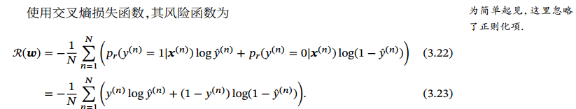
交叉熵损失函数,一般用于分类问题(不仅二分类)
常见的超参数 包括: 聚类算法中的类别个数、 梯度下降法中的步长、 正则化项的系数、神经网络的层数、支持向量机中的核函数等.
提前停止 (Early Stop):如果在验证集上的错误率不再下降,就停止迭代. 可以防止过拟合.
随机梯度下降法 (Stochastic Gradient Descent,SGD):在每次迭代时只采集一个样本, 计算这个样本损失函数的梯度并更新参数.
第 𝑡 次迭代时,随机选取一个包含 𝐾(2的n次方计算效率高) 个样本的子集 𝒮𝑡,计算这个子集上每个样本损失函数的梯度并进行平均,然后再进行参数更新:
批量梯度下降和随机梯度下降之间的区别 :在于每次迭代的优化目标是对所有样本的平均损失函数还是单个样本的损失函数.
共线性 (collinearity):一个特征可以通过其他特征的线性组合来被准确的预测.
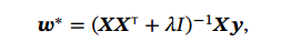
岭回归 (Ridge Regression):给XX^T的对角线元素都加上一个常数𝜆使得 (𝑿𝑿^T + 𝜆𝐼)满秩.
岭回归的解:相当于结构风险最小化准则下的最小二乘法估计,其目标函数是: 最小二乘法 (Least Square Method, LSM):
机器学习任务分为两类:
1.样本的特征向量x和标签y之间存在未知的函数关系.
2.条件概率p(y|x)服从某个未知分布.
最大似然估计 (Maximum Likelihood Estimation,MLE):找到一组参数w使得似然函数p(y|X;w,𝜎)最大,等价于它的对数似然函数 log p(y|X; w, 𝜎) 最大.
贝叶斯估计 (Bayesian Estimation): 一种估计 参数w的后验概率分布的方法,后验 = 先验 × 似然率;p(𝒚|𝑿; 𝒘, 𝜎)为 𝒘的似然函数,p(𝒘; 𝜈)为 𝒘的先验.
最大后验估计 (Maximum A Posteriori Estimation,MAP):最优参数为后验分布中概率密度最高的参数.
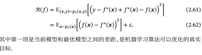
期望错误:理解为错误的平均值
按函数 𝑓(𝒙; 𝜃)的不同,机器学习算法可以分为线性模型和非线性模型;
按照学习准则的不同,机器学习算法也可以分为统计方法和非统计方法. (最常用)按照训练样本提供的信息以及反馈方式的不同,将机器学习算法分为以下几类:
监督学习(Supervised Learning,SL):机器学习的目标是通过建模样本的特征 𝒙 和标签 𝑦 之间的关系𝑦 = 𝑓(𝒙; 𝜃) 或 𝑝(𝑦|𝒙; 𝜃),并且训练集中每个样本都有标签
回归(Regression):标签 𝑦 是连续值(实数或连续整数), 𝑓(𝒙; 𝜃)的输出也是连续值
分类(Classification):标签 𝑦 是离散的类别(符号). 在分类问题中, 学习到的模型也称为分类器(Classifier). 分类问题根据其类别数量又可分为二分类(Binary Classification)和多分类(Multi-class Classification)问题.
图像特征 :将N * M的图像的所有像素存储为N*M向量,也会经常加入一个额外的特征,比如直方图、宽高比、笔画数、纹理特征、边缘特征等.
文字特征 :词袋(Bag-of-Words,BoW)模型,类似one-hot向量.还可以改进为二元特征,即两个词的组合.
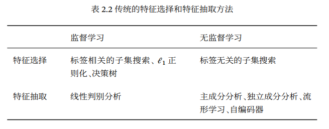
特征学习 (Feature Learning), 也叫表示学习(Representation Learning):如何让机器自动地学习出有效的特征.
特征选择 (Feature Selection):是选取原始特征集合的一个有效子集, 使得 基于这个特征子集训练出来的模型准确率最高.
子集搜索(Subset Search):假设原始特征数为 𝐷, 则共有 2^𝐷 个候选子集. 特征选择的目标是选择一个最优的候选子集.常用的方法是采用贪心的策略: 由空集合开始, 每一轮添加该轮最优的特征,称为前向搜索(Forward Search);或者从原始特征集合开始,每次删除最无用的特征,称为反向搜索(Backward Search).
过滤式方法(Filter Method)不依赖具体的机器学习模型. 每次增加最有信 息量的特征,或删除最没有信息量的特征. 信息量可以通过信息增益(Information Gain)衡量.
包裹式方法(Wrapper Method)是用后续机器学习模型的准确率来评价一 个特征子集. 每次增加对后续机器学习模型最有用的特征,或删除对后续机器学 习任务最无用的特征.将机器学习模型包裹到特征选择过程的内部.
准确率:预测准确的概率.
微平均 是每一个样本的性能指标的算术平均值 . 对于单个样本而言,它的精确率和召回率是相同的(要么都是 1,要么都是 0). 因此精确率的微平均和召回率的微平均是相同的. 同理,F1值的微平均指标是相同的. 当不同类别的样本数量不均衡时,使用宏平均会比微平均更合理些.
实际使用的评估方式:AUC(Area Under Curve)、 ROC(Receiver Operating Characteristic)曲线、PR(Precision-Recall)曲线
ROC曲线:
纵轴是真正例率 (True Positive Rate, 简称TPR,也是召回率): 所有实际为正例中,真的正例的比率.
横轴是假正例率 (False Positive Rate,简称FPR):所有实际为负例中,预测为正例的比率.
ROC曲线作用:
ROC曲线能很容易的查出任意阈值对学习器的泛化性能影响。
有助于选择最佳的阈值。ROC曲线越靠近左上角,模型的查全率就越高。最靠近左上角的ROC曲线上的点是分类错误最少的最好阈值,其假正例和假反例总数最少。
可以对不同的学习器比较性能。将各个学习器的ROC曲线绘制到同一坐标中,直观地鉴别优劣,靠近左上角的ROC曲所代表的学习器准确性最高。
AUC面积作用:衡量二分类模型优劣的一种评价指标,表示预测的正例排在负例前面的概率。
交叉验证 (Cross Validation):把原始数据集平均分为 𝐾 组不重复的子集,每次选 𝐾 − 1组子集作 (𝐾 一般大于 3,可以选10).为训练集,剩下的一组子集作为验证集. 这样可以进行 𝐾 次试验并得到 𝐾 个模型,将这𝐾 个模型在各自验证集上的错误率的平均作为分类器的评价.
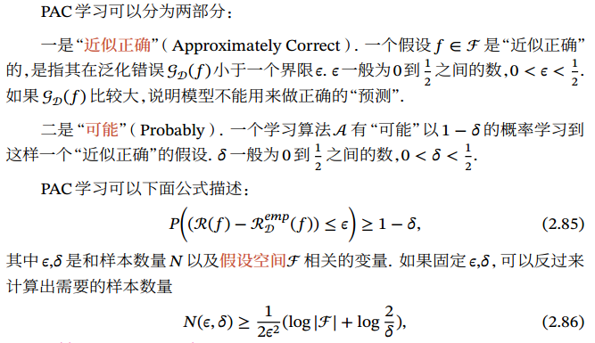
可能近似正确 (Probably Approximately Correct,PAC)学习理论:PAC可学习指该学习算法能够在多项式时间内从合理数量的训练数据 中学习到一个近似正确的;𝑓(𝒙)模型越复杂,需要样本越多;
没有免费的午餐 (No Free Lunch Theorem,NFL):如果一个算法 对某些问题有效,那么它一定在另外一些问题上比纯随机搜索算法更差. 也就是 说,不能脱离具体问题来谈论算法的优劣.
丑小鸭定理 (Ugly Duckling Theorem):“ 丑小鸭与白天鹅之间的区别和两只白天鹅之间的区别一样大”. 世界上不存在分类的客观标准,一切分类的标准都是主观的。
奥卡姆剃刀原理 (Occam’s Razor):“ 如无必要,勿增实体”.简单的模型泛化能力更好. 如果有两个性能相近的模型,我们应该选择更简单的模型. 因此,在机器学习的学习准则上,我们经常会引入参数正则化来限制模型能力,避免过拟合.
奥卡姆剃刀的一种形式化是最小描述长度(Minimum Description Length, MDL)原则:即对一个数据集 𝒟,最好的模型 𝑓 ∈ ℱ 是会使得数据集的压缩效果最好,即编码长度最小.
归纳偏置 (Inductive Bias):经常会对学习的问题做一些假设,在贝叶斯学习中也经常称为先验(Prior).在最近邻分类器中,我们会假设在特征空间中,一个小的局部区域中的大部分样本都同属一类. 在朴素贝叶斯分类器中,我们会假设每个特征的条件概率是互相独立的.
《第七章》 优化:优化算法的目标函数通常是一个基于训练数据集的损失函数,优化的目标在于降低训练误差。
深度学习:深度学习的目标在于降低泛化误差。为了降低泛化误差,除了使用优化算法降低训练误差以外,还需要注意应对过拟合。
梯度接近0时,是为局部最优点或鞍点:由于学习模型参数维度通常是高维,所以鞍点比局部最小值更常见。
《第三章》 《第三章》
线性回归模型 的房屋价格预测表达式为:
假设我们采集的样本数为n,索引为i的样本的特征为x(i)1 和x(i)2 ,标签为y(i) 。对于索引为i的房屋,w指权重(weight),b是偏差(bias),y帽是预估。
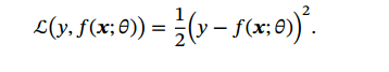
平方损失函数
《第六章》 语言模型 (language model)是自然语言处理的重要技术。自然语言处理中最常见的数据是文本数据。我们可以把一段自然语言文本看作一段离散的时间序列。
可以计算为w1,w2两词相邻的频率与w1词频的比值,因为该比值即P(w1,w2)与P(w1)之比
P(w3∣w1,w2)同理可以计算为w1、w2和w3这3个词相邻的频率与w1和w2这2个词相邻的频率的比值。
复制 torch.empty(5, 3)
torch.rand(5, 3)
torch.zeros(5, 3, dtype=torch.long)
torch.tensor([5.5, 3]) # 根据数组创建
# 获取形状
print(x.size())
print(x.shape)
复制 x + y
torch.add(x, y)
y.add_(x) # 就地加法,类似x.copy_(y), x.t_()
复制 # 不同的size,但是是共享data
y = x.view(15)
z = x.view(-1, 5) # -1所指的维度可以根据其他维度的值推出来
print(x.size(), y.size(), z.size())
# torch.Size([5, 3]) torch.Size([15]) torch.Size([3, 5])
# 不同size,不同data的新副本
x_cp = x.clone().view(15) # clone会被记录在计算图中,即梯度传播影响源数据
# reshape() 不保证返回的一定是拷贝后的数据
复制 x = torch.randn(1)
print(x)
print(x.item())
# tensor([2.3466])
# 2.3466382026672363
复制 y[:] = y + x # 就地
y = y + x # 非就地
# view只是共享了tensor的数据,二者id(内存地址)并不一致。
# 因为tensor里面还有除了data的数据
复制 # tensor to numpy
a = torch.ones(5)
b = a.numpy()
复制 # numpy to tensor
import numpy as np
a = np.ones(5)
b = torch.from_numpy(a)
# torch.tensor()将NumPy数组转换成Tensor
# 该方法总是会进行数据拷贝
c = torch.tensor(a)
复制 import matplotlib.pyplot as plt
import numpy as np
# 展示图片
def imshow(img):
img = img / 2 + 0.5 # 逆归一化
npimg = img.numpy()
plt.imshow(np.transpose(npimg, (1, 2, 0)))
plt.show()
# 获取一些图片
dataiter = iter(trainloader)
images, labels = dataiter.next()
print(images.size())
imshow(torchvision.utils.make_grid(images))
print(' '.join('%5s' % classes[labels[j]] for j in range(4)))
复制 torch.Size([4, 3, 32, 32])
复制 import torch.nn as nn
import torch.nn.functional as F
class Net(nn.Module):
def __init__(self):
super(Net, self).__init__()
self.conv1 = nn.Conv2d(3, 6, 5)
self.pool = nn.MaxPool2d(2, 2)
self.conv2 = nn.Conv2d(6, 16, 5)
self.fc1 = nn.Linear(16 * 5 * 5, 120)
self.fc2 = nn.Linear(120, 84)
self.fc3 = nn.Linear(84, 10)
def forward(self, x):
x = self.pool(F.relu(self.conv1(x)))
x = self.pool(F.relu(self.conv2(x)))
x = x.view(-1, 16 * 5 * 5)
x = F.relu(self.fc1(x))
x = F.relu(self.fc2(x))
x = self.fc3(x)
return x
net = Net()
print(net)
复制 Net(
(conv1): Conv2d(3, 6, kernel_size=(5, 5), stride=(1, 1))
(pool): MaxPool2d(kernel_size=2, stride=2, padding=0, dilation=1, ceil_mode=False)
(conv2): Conv2d(6, 16, kernel_size=(5, 5), stride=(1, 1))
(fc1): Linear(in_features=400, out_features=120, bias=True)
(fc2): Linear(in_features=120, out_features=84, bias=True)
(fc3): Linear(in_features=84, out_features=10, bias=True)
)
复制 import torch.optim as optim
criterion = nn.CrossEntropyLoss() # 交叉熵
optimizer = optim.SGD(net.parameters(), lr=0.001, momentum=0.9) # 设置了动量的SGD
复制 for epoch in range(2):
running_loss = 0.0
for i, data in enumerate(trainloader, 0): # 从下标0开始迭代
inputs, labels = data # 读取数据
optimizer.zero_grad() # 初始梯度
outputs = net(inputs) # 前向传播
loss = criterion(outputs, labels) # 计算交叉熵
loss.backward() # 反向传播
optimizer.step() # 优化算法,学习参数
running_loss += loss.item()
if i % 2000 == 1999:
print('[%d, %5d] loss: %.3f' %
(epoch + 1, i + 1, running_loss / 2000))
running_loss = 0.0
print('Finished Training')
复制 [1, 2000] loss: 2.193
[1, 4000] loss: 1.864
[1, 6000] loss: 1.660
[1, 8000] loss: 1.559
[1, 10000] loss: 1.514
[1, 12000] loss: 1.468
[2, 2000] loss: 1.384
[2, 4000] loss: 1.356
[2, 6000] loss: 1.325
[2, 8000] loss: 1.317
[2, 10000] loss: 1.295
[2, 12000] loss: 1.271
Finished Training
复制 PATH = './cifar_net.pth'
torch.save(net.state_dict(), PATH) # 保存字典到指定文件
复制 dataiter = iter(testloader)
images, labels = dataiter.next()
imshow(torchvision.utils.make_grid(images))
print(' '.join('%5s' % classes[labels[j]] for j in range(4)))
复制 net = Net()
net.load_state_dict(torch.load(PATH))# 先加载数据,再将数据加载到net里,非必须
复制 <All keys matched successfully>
复制 outputs = net(images) # 使用训练后的数据,进行预测输出
_, predicted = torch.max(outputs, 1) # torch.max(data, dim)获取dim维向量的最大值,返回value,index
print('Predicted: ', ' '.join('%5s' % classes[predicted[j]]
for j in range(4)))
复制 Predicted: cat car ship plane
复制 correct = 0
total = 0
with torch.no_grad():
for data in testloader:
images, labels = data
outputs = net(images)
_, predicted = torch.max(outputs.data, 1)
total += labels.size(0)
correct += (predicted == labels).sum().item()
print('Accuracy of the network on the 10000 test images: %d %%' % (
100 * correct / total))
复制 Accuracy of the network on the 10000 test images: 54 %
复制 class_correct = list(0. for i in range(10)) # 10个 0.
class_total = list(0. for i in range(10))
with torch.no_grad():
for data in testloader:
images,labels = data
outputs = net(images)
_, predicted = torch.max(outputs, 1)
c = (predicted==labels).squeeze() # 将结果压缩一个维度
for i in range(4): # 批量为4
label = labels[i]
class_correct[label] += c[i].item()
class_total[label] += 1
for i in range(10):
print('Accuracy of %5s : %2d %%' % (
classes[i], 100 * class_correct[i] / class_total[i]))
复制 Accuracy of plane : 57 %
Accuracy of car : 52 %
Accuracy of bird : 41 %
Accuracy of cat : 44 %
Accuracy of deer : 27 %
Accuracy of dog : 40 %
Accuracy of frog : 69 %
Accuracy of horse : 56 %
Accuracy of ship : 77 %
Accuracy of truck : 75 %
复制 device = torch.device("cuda:0" if torch.cuda.is_available() else "cpu")
print(device)
复制 net.to(device) # 所有的模块和参数都会递归的变成CUDA张量
inputs, labels = data[0].to(device), data[1].to(device) # 所有数据都需要在GPU normal(mean,std)/uniform(from,to)
Leetcode 根据不同题目的标签,先从简单题刷起,最开始尽可能做,后面可能速度降下来。
可以的话每天三题左右。
能翻墙就翻墙吧,然后不要乱配置源,保持原始的就可以了,有些包在国内版本比较低,有冲突。
学会使用conda管理包,以及查看下载包时候出现的异常,尤其是标红的,很重要,不要轻易忽略,不然就是下一个坑。
jupyter lab也挺好用的,但是第一次使用,由于各个包版本没有搞好,导致404无法连接服务器,也就无法运行python,原因如第4点所说。
吐槽一下,在使用jupyter时候,好像不能同时打开同一个虚拟环境的另一个命令行,也就难以同时进行包管理。或者是我打开方式不对?
size——元素总数
zeros默认置零,ones默认置1,记得因为复数,有s
array——多维数组最普通的定义方式,array()括号里的即为数组
nd.random.normal(a,b,shape=(3,4))——random指随机,normal指正态分布,a-b范围
+-*/,还有==,都是逐个元素进行的。exp(),dot()也是,其中dot记得通过X.T转置
concat(X,Y,dim=0),将第0个维度(shape中的第0个元素)保持不变,其他结合起来。
sum()——获得所有元素的和,list内一个浮点数
norm()——逐个元素的平方之和后开根号=欧几里得范数(长度)=L2范数(长度),是list
asscalar()——as scalar,作为标量,即list-->num
broadcasting,广播机制——犹如C语言中的类型自动转换,将多维数组的长度扩大到可以进行运算,以保证运算的正确性。经测试发现,只有一行或者一列才可以广播,此时无歧义。
内存不变的操作:Z[:] = X + Y;nd.elemwise_add(X, Y, out=Z);X += Y; X[:] = X + Y
Y = Y + X; 会新开内存Y和临时内存X+Y
nd.array(P)——转换numpy-->NDArray
D.asnumpy()——转换NDArray-->numpy
替换成其他形状,结果是否和预期一样?
复制 from mxnet import autograd, nd
x = nd.arange(4).reshape((4, 1))
# 申请梯度的内存
x.attach_grad()
# 在运算的过程中记录梯度,此时从预测模式转为训练模式
with autograd.record():
y = 2 * nd.dot(x.T, x)
# 求梯度,y如果不是标量会求和
y.backward()
似然函数理解:它是给定联合样本值x下关于(未知)参数θ的函数,也就是将x作为常数,关于参数的函数.
Hinge损失函数,适用于二分类,y为-1或1.
符号定义 : [ x ] + = m a x ( 0 , x ) 符号定义:[x]_+=max(0,x) 符号定义 : [ x ] + = ma x ( 0 , x )
结构化学习(Structured Learning):问题的输出 𝒚通常是结构化的对象,比如序列、树或图等.
无监督学习(Unsupervised Learning,UL):指从不包含目标标签的训练样本中自动学习到一些有价值的信息. 典型的无监督学习问题有聚类、密度估计、特征学习、降维等
强化学习(Reinforcement Learning, RL)是一类通过交互来学习的机器学习算法. 在强化学习中,智能体根据环境的状态做出一个动作,并得到即时或延时的奖励. 智能体在和环境的交互中不断学习并调整策略,以取得最大化的期望总回报.
ℓ1 正则化: 通过 ℓ1 正则化来实现特征选择. 由于 ℓ1 正则化会导致稀疏特征,因此间接实现了特征选择. 特征抽取 (Feature Extraction):可以分为监督和无监督的方法. 监督的特征学习的目标是抽取对一个特定的预测任务最有用的特征,比如线性判别分析(Linear Discriminant Analysis,LDA). 而无监督的特征学习和具体任务无关,其目标通常是减少冗余信息和噪声,比如主成分分析(Principal Component Analysis,PCA). 维度灾难 (Curse of Dimensionality). 深度学习(Deep Learning, DL):如果我们将特征的表示学习和机器学习的预测学习有机地统一到一个模型中,建立一个端到端的学习算法,就可以有效地避免它们之间准则的不一致性. 目前比较有效的模型是神经网络,即将最后的输出层作为预测学习,其他层作为表示学习.
目标函数 = ∑ (观测值 − 理论值 ) 2 目标函数 = \sum\limits(观测值-理论值)^2 目标函数 = ∑ (观测值 − 理论值 ) 2
卷积运算:与互相关运算类似。为了得到卷积运算的输出,我们只需将核数组左右翻转并上下翻转,再与输入数组做互相关运算。可见,卷积运算和互相关运算虽然类似,但如果它们使用相同的核数组,对于同一个输入,输出往往并不相同。
特征图(feature map):二维卷积层输出的二维数组可以看作输入在空间维度(宽和高)上某一级的表征。
x的感受野(receptive field):影响元素x的前向计算的所有可能输入区域(可能大于输入的实际尺寸)。
corr2d因为用了[i,j]=导致自动求导失败,这是由于autograd目前还有局限性。在该类的forward函数里,将corr2d函数替换成nd.Convolution类使得自动求梯度变得可行。
构造一个输入图像X,令它有水平方向的边缘。如何设计卷积核K来检测图像中水平边缘?如果是对角方向的边缘呢?
答:检测水平边缘的核函数应该是[[1],[-1]];对角方向的核函数[1, -1]或[[1],[-1]]或[[1, 0],[-1, 0]];
对角方向的边缘监测方法有按水平的,按垂直的,或者都要。根据不同的方法,宽高会发生相应变化。
试着对我们自己构造的Conv2D类进行自动求梯度,会有什么样的错误信息?在该类的forward函数里,将corr2d函数替换成nd.Convolution类使得自动求梯度变得可行。
答:infershape[attrs.op](attrs, &in_shapes, &out_shapes)
corr2d因为用了[i,j]=导致自动求导失败,这是由于autograd目前还有局限性。改成 nd.Convolution 会没问题,因为它手动实现了backward函数。
如何通过变化输入和核数组将互相关运算表示成一个矩阵乘法?
答:卷积变成矩阵乘法,从乘法和加法的运算次数上看,两者没什么差别,但是转化成矩阵后,运算时需要的数据被存在连续的内存上,这样访问速度大大提升。
方法参考如下:https://www.cnblogs.com/marsggbo/p/12074297.html
如何构造一个全连接层来进行物体边缘检测?
答:全连接层是指使用nn.Dense?
填充(padding)是指在输入高和宽的两侧填充元素(通常是0元素)。
在输入的高和宽两侧分别填充了0元素的二维互相关计算 步幅(stride):我们将每次滑动的行数和列数。输出第一列第二个元素时,卷积窗口向下滑动了3行,而在输出第一行第二个元素时卷积窗口向右滑动了2列。当卷积窗口在输入上再向右滑动2列时,由于输入元素无法填满窗口,无结果输出。
对本节最后一个例子通过形状计算公式来计算输出形状,看看是否和实验结果一致。
一致,分别是8/3和8/4的下取整。
通道(channel)维:例如,彩色图像在高和宽2个维度外还有RGB(红、绿、蓝)3个颜色通道。称其通道维为3.
多输出通道:每个输出通道上的结果由卷积核在该输出通道上的核数组 与整个输入数组 计算而来。
卷积窗口形状为1×1(k_h=k_w=1)的多通道卷积层。
假设我们将通道维当作特征维,将高和宽维度上的元素当成数据样本,那么1×1卷积层的作用与全连接层等价。
假设输入形状为ci×h×w,且使用形状为co×ci×kh×kw、填充为(ph,pw)、步幅为(sh,sw)的卷积核。那么这个卷积层的前向计算分别需要多少次乘法和加法?
答:
输出形状为:
c o × ⌊ ( n h − k h + p h + s h ) / s h ⌋ × ⌊ ( n w − k w + p w + s w ) / s w ⌋ c_o\times\lfloor(n_h-k_h+p_h+s_h)/s_h\rfloor \times \lfloor(n_w-k_w+p_w+s_w)/s_w\rfloor c o × ⌊( n h − k h + p h + s h ) / s h ⌋ × ⌊( n w − k w + p w + s w ) / s w ⌋ 乘法次数:
k h × k w × c o × ⌊ ( n h − k h + p h + s h ) / s h ⌋ × ⌊ ( n w − k w + p w + s w ) / s w ⌋ k_h\times k_w \times c_o\times\lfloor(n_h-k_h+p_h+s_h)/s_h\rfloor \times \lfloor(n_w-k_w+p_w+s_w)/s_w\rfloor k h × k w × c o × ⌊( n h − k h + p h + s h ) / s h ⌋ × ⌊( n w − k w + p w + s w ) / s w ⌋ 加法次数:
[ ( k h × k w ) 个数连加 ] × ( c i 个数连加 ) × ⌊ ( n h − k h + p h + s h ) / s h ⌋ × ⌊ ( n w − k w + p w + s w ) / s w ⌋ [(k_h\times k_w)个数连加]\times(c_i个数连加)\times\lfloor(n_h-k_h+p_h+s_h)/s_h\rfloor \times \lfloor(n_w-k_w+p_w+s_w)/s_w\rfloor [( k h × k w ) 个数连加 ] × ( c i 个数连加 ) × ⌊( n h − k h + p h + s h ) / s h ⌋ × ⌊( n w − k w + p w + s w ) / s w ⌋ 翻倍输入通道数ci和输出通道数co会增加多少倍计算?翻倍填充呢?
答:通过上述公式可以看出,翻倍导致增加的计算程度大致为:c_o > c_i > p_h(p_w)
如果卷积核的高和宽kh=kw=1,能减少多少计算?
答:乘法降低至1/(k_h乘k_w),加法降低至1/(k_w*k_h-1)
本节最后一个例子中的变量Y1和Y2完全一致吗?原因是什么?
答:不完全一致,一个是通过矩阵乘法的方式、一个是通过互相关计算。某个地方的精度不一样,比如说没有批量求和。
当卷积窗口不为1×1时,如何用矩阵乘法实现卷积计算?
答:将卷积窗口reshape为行向量或者列向量。
池化层:池化层每次对输入数据的一个固定形状窗口(又称池化窗口)中的元素计算输出。池化层直接计算池化窗口内元素的最大值或者平均值。该运算也分别叫做最大池化或平均池化。
池化窗口形状为\ :math:2\times 2\ 的最大池化 池化层的一个主要作用是缓解卷积层对位置的过度敏感性。(把数组按局部矩阵最大值或者局部矩阵平均值缩小)
分析池化层的计算复杂度。假设输入形状为c×h×w,我们使用形状为ph×pw的池化窗口,而且使用(ph,pw)填充和(sh,sw)步幅。这个池化层的前向计算复杂度有多大?
答:时间复杂度为
c × ⌊ ( h − k h + p h + s h ) / s h ⌋ × ⌊ ( w − k w + p w + s w ) / s w ⌋ × ( m a x 的时间 ) c×⌊(h−k_h+p_h+s_h)/s_h⌋×⌊(w−k_w+p_w+s_w)/s_w⌋×(max的时间) c × ⌊( h − k h + p h + s h ) / s h ⌋ × ⌊( w − k w + p w + s w ) / s w ⌋ × ( ma x 的时间 ) 想一想,最大池化层和平均池化层在作用上可能有哪些区别?
答:平均池化可以提取背景信息,减少冲击失真,模糊,平滑。最大池化可以提取特征纹理,增强图片亮度
觉得最小池化层这个想法有没有意义?
答:因为像素值为正数决定的,0代表为黑色。采用最小池化很可能全部都是0。最小池化甚至会让你的神经网络轻易过拟合甚至无法训练。
卷积层块里的基本单位是卷积层后接最大池化层 :卷积层用来识别图像里的空间模式,如线条和物体局部,之后的最大池化层则用来降低卷积层对位置的敏感性。卷积层块由两个这样的基本单位重复堆叠构成。
LeNet交替使用卷积层和最大池化层后接全连接层来进行图像分类。
尝试基于LeNet构造更复杂的网络来提高分类准确率。例如,调整卷积窗口大小、输出通道数、激活函数和全连接层输出个数。在优化方面,可以尝试使用不同的学习率、初始化方法以及增加迭代周期。
答:1.换成relu激活函数显著提高。2.第二个卷积层的通道可以适当减少。神经网络定义如上,其他超参数如下。
LeNet的优缺点:小数据集成绩不错,但在大数据集上表现不尽人意。
尝试增加迭代周期。跟LeNet的结果相比,AlexNet的结果有什么区别?为什么?
答:AlexNet的训练时间长了三倍,训练结果精确度提高了10%左右。AlexNet精确率提高的慢一点。应该是用了dropout以及lr比较低的原因。同时神经网络复杂度大大提高。
AlexNet对Fashion-MNIST数据集来说可能过于复杂。试着简化模型来使训练更快,同时保证准确率不明显下降。
答:看5.5章我的笔记中的改进后的LeNet。个人以为,改为relu激活就能显著提高精确率了,对于Fashion-MNIST而言。
修改批量大小,观察准确率和内存或显存的变化。
答:批量改成256,准确率降低。显存没有看出显著变化。可能观测方法有问题,只是通过任务管理器的性能来查看。
VGG块的组成规律是:连续使用数个相同的填充为1、窗口形状为3×3的卷积层后接上一个步幅为2、窗口形状为2×2的最大池化层。卷积层保持输入的高和宽不变,而池化层则对其减半。
与AlexNet相比,VGG通常计算慢很多,也需要更多的内存或显存。试分析原因。
答:通道更多,刚开始时候的宽高更大。
尝试将Fashion-MNIST中图像的高和宽由224改为96。这在实验中有哪些影响?
答:时间缩短到了1/4,精确率略低于224的。
参考VGG论文里的表1来构造VGG其他常用模型,如VGG-16和VGG-19 [1]。
下图是AlexNet和VGG的网络结构局部和NiN的网络结构局部的对比:
左图是AlexNet和VGG的网络结构局部,右图是NiN的网络结构局部 1×1卷积层。它可以看成全连接层。其中空间维度(高和宽)上的每个元素相当于样本,通道相当于特征。
调节超参数,提高分类准确率。
答:1.通过提高迭代次数可以提高准确率。2.降低dropout的值至0.3能有效提高准确率。
batch_size过大会内存溢出。lr降低或提高均无显著效果。
为什么NiN块里要有两个1×1卷积层?去除其中的一个,观察并分析实验现象。
答:第一个1x1卷积层实现feature map的提取,第二个1x1卷积层进行feature map的组合
现象:1.时间降低。因为模型复杂度降低。2.第二轮的精确率下降了。3.最终精确率低。
原因可能是少了一个卷积层导致了feature map没有组合在一起,从而缺少了一部分的特征。直接通过feature map来回归参数。
feature map:在每个卷积层,数据都是以三维形式存在的。你可以把它看成许多个二维图片叠在一起,其中每一个称为一个feature map。
前3条线路使用窗口大小分别是1×1、3×3和5×5的卷积层来抽取不同空间尺寸下的信息,其中中间2个线路会对输入先做1×1卷积来减少输入通道数,以降低模型复杂度。
第四条线路则使用3×3最大池化层,后接1×1卷积层来改变通道数。
4条线路都使用了合适的填充来使输入与输出的高和宽一致 。
最后我们将每条线路的输出在通道维上连结,并输入接下来的层中去。
对比AlexNet、VGG和NiN、GoogLeNet的模型参数尺寸。为什么后两个网络可以显著减小模型参数尺寸?
NiN:去掉了AlexNet最后的3个全连接层,取而代之地,NiN使用了输出通道数等于标签类别数的NiN块,然后使用全局平均池化层对每个通道中所有元素求平均并直接用于分类。NiN的这个设计的好处是可以显著减小模型参数尺寸,从而缓解过拟合。
GoogLeNet:其中中间2个线路会对输入先做1×1卷积来减少输入通道数,以降低模型复杂度。另外,Inception块中可以自定义的超参数是每个层的输出通道数,我们以此来控制模型复杂度。
第一步:首先,对小批量BB求均值和方差,其中平方计算是按元素求平方。
第二步:接下来,使用按元素开方和按元素除法对x(i)标准化,ϵ>0是一个很小的常数,保证分母大于0。
第三步:引入两个可学习参数,拉伸(scale)参数 γ和偏移(shift)参数 β,如果批量归一化无益,学出的模型可以不使用批量归一化。两个参数和x(i)形状相同为d维向量。它们与x(i)分别做按元素乘法(符号⊙)和加法计算:
**卷积层的批量归一化:**批量归一化发生在卷积计算之后、应用激活函数之前。如果卷积计算输出多个通道,我们需要对这些通道的输出分别做批量归一化,且每个通道都拥有独立的拉伸和偏移参数,并均为标量。
**预测时的批量归一化:**训练时,我们可以将批量大小设得大一点。预测时,一种常用的方法是通过移动平均估算整个训练数据集的样本均值和方差,并在预测时使用它们得到确定的输出。ps:移动平均法arrow-up-right
在模型训练时,批量归一化利用小批量上的均值和标准差,不断调整神经网络的中间输出,从而使整个神经网络在各层的中间输出的数值更稳定。
批量归一化层和丢弃层一样,在训练模式和预测模式的计算结果是不一样的。
能否将批量归一化前的全连接层或卷积层中的偏差参数去掉?为什么?(提示:回忆批量归一化中标准化的定义。)
答:不行,为了使得均值为0、标准差为1。
尝试将批量归一化层插入LeNet的其他地方,观察并分析结果的变化。
答:将批量归一化插入到激活函数之后,跟训练集的拟合效果更好了。先通过激活函数过滤了一些数据,所以拟合效果更好了。batchnorm主要是让收敛变快,但对acc影响不大。
尝试一下不学习拉伸参数gamma和偏移参数beta(构造的时候加入参数grad_req='null'来避免计算梯度),观察并分析结果。
答:结果acc略低于原来的1%左右,因为归一化不一定有益,需要通过学习拉伸参数和偏移参数来使其达到最佳的程度。
查看BatchNorm类的文档来了解更多使用方法,例如,如何在训练时使用基于全局平均的均值和方差。
答:nn.BatchNorm(use_global_stats=True)可以设置使用全局。
设输入为x。假设图中最上方激活函数输入的理想映射为f(x)。
右图虚线框中的部分需要拟合出有关恒等映射的残差映射f(x)−x
残差块通过跨层的数据通道从而能够训练出有效的深度神经网络。
参考ResNet论文的表1来实现不同版本的ResNet [1]。
对于比较深的网络, ResNet论文中介绍了一个“瓶颈”架构来降低模型复杂度。尝试实现它 [1]。
答:”For each residual function F, we use a stack of 3 layers instead of 2 (Fig. 5). The three layers are 1×1, 3×3, and 1×1 convolutions, where the 1×1 layers are responsible for reducing and then increasing (restoring) dimensions, leaving the 3×3 layer a bottleneck with smaller input/output dimensions.“
未实现,思路是:修改resnet_block函数设置1×1, 3×3, and 1×1 的三个卷积层。
在ResNet的后续版本里,作者将残差块里的“卷积、批量归一化和激活”结构改成了“批量归一化、激活和卷积”,实现这个改进([2],图1)。
DenseNet论文中提到的一个优点是模型参数比ResNet的更小,这是为什么?
答:ResNet里通过步幅为2的残差块在每个模块之间减小高和宽。DenseNet使用过渡层来减半高和宽,并减半通道数。
DenseNet被人诟病的一个问题是内存或显存消耗过多。真的会这样吗?可以把输入形状换成224×224,来看看实际的消耗。
答:cudaMalloc failed: out of memory
实现DenseNet论文中的表1提出的不同版本的DenseNet [1]。
答:
若输入矩阵 : n h × n w 且卷积核 : k h × k w 则输出形状 : ( n h − k h + 1 ) × ( n w − k w + 1 ) 若输入矩阵:n_h\times n_w\\ 且卷积核:k_h\times k_w\\ 则输出形状:(n_h-k_h+1) \times (n_w-k_w+1) 若输入矩阵 : n h × n w 且卷积核 : k h × k w 则输出形状 : ( n h − k h + 1 ) × ( n w − k w + 1 ) 若高填充 p h 行,宽填充 p w 行,则输出形状 ( n h − k h + p h + 1 ) × ( n w − k w + p w + 1 ) 可以设置 p h = k h − 1 , p w = k w − 1 使得输入和输出形状一致。 若高填充p_h行,宽填充p_w行,则输出形状(n_h-k_h+p_h+1)\times(n_w-k_w+p_w+1)\\ 可以设置p_h=k_h-1,p_w=k_w-1使得输入和输出形状一致。 若高填充 p h 行,宽填充 p w 行,则输出形状 ( n h − k h + p h + 1 ) × ( n w − k w + p w + 1 ) 可以设置 p h = k h − 1 , p w = k w − 1 使得输入和输出形状一致。 当高上步幅为 s h ,宽上步幅为 s w 时,输出形状为 : ⌊ ( n h − k h + p h + s h ) / s h ⌋ × ⌊ ( n w − k w + p w + s w ) / s w ⌋ 如果设置 p h = k h − 1 和 p w = k w − 1 ,那么输出形状将简化为 : ⌊ ( n h + s h − 1 ) / s h ⌋ × ⌊ ( n w + s w − 1 ) / s w ⌋ 更进一步,如果输入的高和宽能分别被高和宽上的步幅整除,那么输出形状将是 ( n h / s h ) × ( n w / s w ) 。 当高上步幅为s_h ,宽上步幅为s_w 时,输出形状为:\\ \lfloor(n_h-k_h+p_h+s_h)/s_h\rfloor \times \lfloor(n_w-k_w+p_w+s_w)/s_w\rfloor\\如果设置 p_h=k_h−1 和 p_w=k_w−1 ,那么输出形状将简化为 :\\⌊(n_h+s_h−1)/s_h⌋×⌊(n_w+s_w−1)/s_w⌋ \\ 更进一步,如果输入的高和宽能分别被高和宽上的步幅整除,那么输出形状将是 (n_h/s_h)×(n_w/s_w) 。 当高上步幅为 s h ,宽上步幅为 s w 时,输出形状为 : ⌊( n h − k h + p h + s h ) / s h ⌋ × ⌊( n w − k w + p w + s w ) / s w ⌋ 如果设置 p h = k h − 1 和 p w = k w − 1 ,那么输出形状将简化为 : ⌊( n h + s h − 1 ) / s h ⌋ × ⌊( n w + s w − 1 ) / s w ⌋ 更进一步,如果输入的高和宽能分别被高和宽上的步幅整除,那么输出形状将是 ( n h / s h ) × ( n w / s w ) 。
μ B ← 1 m ∑ i = 1 m x ( i ) , σ B 2 ← 1 m ∑ i = 1 m ( x ( i ) − μ B ) 2 , \boldsymbol{\mu}_\mathcal{B} \leftarrow \frac{1}{m}\sum_{i = 1}^{m} \boldsymbol{x}^{(i)},\\\boldsymbol{\sigma}_\mathcal{B}^2 \leftarrow \frac{1}{m} \sum_{i=1}^{m}(\boldsymbol{x}^{(i)} - \boldsymbol{\mu}_\mathcal{B})^2, μ B ← m 1 i = 1 ∑ m x ( i ) , σ B 2 ← m 1 i = 1 ∑ m ( x ( i ) − μ B ) 2 , x ^ ( i ) ← x ( i ) − μ B σ B 2 + ϵ , \hat{\boldsymbol{x}}^{(i)} \leftarrow \frac{\boldsymbol{x}^{(i)} - \boldsymbol{\mu}_\mathcal{B}}{\sqrt{\boldsymbol{\sigma}_\mathcal{B}^2 + \epsilon}}, x ^ ( i ) ← σ B 2 + ϵ x ( i ) − μ B , y ( i ) ← γ ⊙ x ^ ( i ) + β . {\boldsymbol{y}}^{(i)} \leftarrow \boldsymbol{\gamma} \odot \hat{\boldsymbol{x}}^{(i)} + \boldsymbol{\beta}. y ( i ) ← γ ⊙ x ^ ( i ) + β .
当函数的海森矩阵在梯度为0的位置上的特征值全为正时,该函数得到局部最小值。
当函数的海森矩阵在梯度为0的位置上的特征值全为负时,该函数得到局部最大值。
当函数的海森矩阵在梯度为0的位置上的特征值有正有负时,该函数得到鞍点。
对于k维参数,第一种的概率是0.5^k。显然鞍点的概率大。
低维空间的非凸优化问题:主要是存在一些局部最优点。采用梯度下降方法时,不合适的参数初始化会导致陷入局部最优点,因此主要的难点是如何选择初始化参数和逃离局部最优点。 高维空间中非凸优化的难点:并不在于如何逃离局部最优点,而是如何逃离鞍点。鞍点(saddle point)是梯度为0,但是在一些维度上是最高点,在另一些维度上是最低点。
对于深度学习中的优化问题,你还能想到哪些其他的挑战?
答:学习率的调整,如何选择初始化参数。
numpy.meshgrid()——生成网格点坐标矩阵
举例:X轴可以取三个值1,2,3, Y轴可以取三个值7,8, 请问可以获得多少个点的坐标?
学习率过大或过小都有问题。一个合适的学习率通常是需要通过多次实验找到的。
当训练数据集的样本较多时,梯度下降每次迭代的计算开销较大O(n),因而随机梯度下降通常更受青睐O(1)。理解:梯度下降需要梯度求和后取平均,随机梯度下降只采样一个来计算梯度。
使用一个不同的目标函数,观察梯度下降和随机梯度下降中自变量的迭代轨迹。
答:梯度下降比较线性,随机梯度下降比较曲折。
在二维梯度下降的实验中尝试使用不同的学习率,观察并分析实验现象
答:小于0.5的还可以用,超过的无法收敛。学习率偏低会导致无法接近0点,稍高会在0点附近徘徊,过高则不收敛。猜测过高导致了接近指数爆炸的效果。
小批量随机梯度下降中每次迭代的计算开销为O(|B|)。
当批量大小等于训练数据样本数时,该算法即梯度下降。
修改批量大小和学习率,观察目标函数值的下降速度和每个迭代周期的耗时。
答:批量小,每个迭代周期耗时长,下降速度快。近似随机梯度下降。
学习率提高,梯度下降速度越快,每个迭代周期耗时不影响。
查阅MXNet文档,使用Trainer类的set_learning_rate函数,令小批量随机梯度下降的学习率每过一个迭代周期减小到原值的1/10。
答:在迭代周期的循环中添加如下代码。
换句话说,相比于小批量随机梯度下降,动量法在每个时间步的自变量更新量近似于将前者对应的最近1/(1−γ)个时间步 的更新量做了指数加权移动平均后再除以1−γ。所以,在动量法中,自变量在各个方向上的移动幅度不仅取决于当前梯度,还取决于过去的各个梯度在各个方向上是否一致。这样,我们就可以使用较大的学习率,从而使自变量向最优解更快移动
动量γ=0.5,则是1/(1-γ)=2倍小批量梯度下降。
动量γ=0.9,则是1/(1-γ)=10倍小批量梯度下降。
后者是前者五倍,直觉上,后者学习率应该是前者1/5.
使用其他动量超参数和学习率的组合,观察并分析实验结果。
答:momentum越小,结果越不陡。原因:动量越小,相当于越小批量的梯度下降,所以损失降低慢。其他组合改变如上述笔记。
AdaGrad算法,它根据自变量在每个维度的梯度值的大小来调整各个维度上的学习率,从而避免统一的学习率难以适应所有维度的问题。
AdaGrad算法在迭代过程中不断调整学习率,并让目标函数自变量中每个元素都分别拥有自己的学习率。
使用AdaGrad算法时,自变量中每个元素的学习率在迭代过程中一直在降低(或不变)。(AdaGrad算法在迭代后期由于学习率过小,可能较难找到一个有用的解。)
在介绍AdaGrad算法的特点时,我们提到了它可能存在的问题。你能想到什么办法来解决这个问题?
答:AdaGrad算法在迭代后期由于学习率过小,可能较难找到一个有用的解。解决办法:学习率降低的慢一点?指数加权移动平均。
在实验中尝试使用其他的初始学习率,结果有什么变化?
答:损失函数变得曲折了起来。
MSProp算法使用了小批量随机梯度按元素平方的指数加权移动平均来调整学习率。改进了AdaGrad算法。
因为RMSProp算法的状态变量s_t是对平方项g_t⊙g_t的指数加权移动平均,所以可以看作最近1/(1−γ)个时间步的小批量随机梯度平方项的加权平均。
在同样的学习率下,RMSProp算法可以更快逼近最优解。
把γ的值设为1,实验结果有什么变化?为什么?
答:损失函数发散扩大,而后Maximum allowed size exceeded。即获得nan。因为一开始的s_t为0,一直没有增长。后面学习率η除以ε的开根号,所得的值,导致自变量降低很大。
试着使用其他的初始学习率和γ超参数的组合,观察并分析实验结果。
答:原来:初始学习率0.01 和γ超参数0.9
修改1:初始学习率0.01 和γ超参数0.99-------结果:损失函数比原来更快下降。因为s_t变小,所以学习率更容易变大。
修改2:初始学习率0.05 和γ超参数0.90-------结果:损失函数比原来更快下降,后期更曲折,有增有减。因为η变大,所以学习率更容易变大。后期由于学习率还是增大,所以变得曲折。
小批量随机梯度g_t按元素平方的指数加权移动平均变量s_t
状态变量Δx_t,在时间步0时被初始化为0。记录自变量变化量g′t按元素平方的指数加权移动平均。
AdaDelta算法没有学习率超参数,它通过使用有关自变量更新量平方的指数加权移动平均的项
调节AdaDelta算法中超参数ρ的值,观察实验结果。
答:有点类似学习率,增大就容易降低损失。但是直觉上觉得,比学习率更稳定可靠。
小批量随机梯度gt按元素平方 的指数加权移动平均变量st
注:之前AdaDelta算法是只有按元素平方的,而Adam是增加了没有平方的小批量随机梯度也做指数加权移动平均。
Adam算法在RMSProp算法的基础上对小批量随机梯度 也做了指数加权移动平均。
调节学习率,观察并分析实验结果。
答:高于0.03就效果不太好了,迭代后期产生了曲折变化。原因想不明白。目前来看,Adam的学习率应当低一点
有人说Adam算法是RMSProp算法与动量法的结合。想一想,这是为什么?
答:因为对小批量随机梯度做指数加权移动平均就是动量法。
输入是 n 维向量 x = [ x 1 , x 2 , … , x n ] ⊤ 海森矩阵 H = [ ∂ 2 f ∂ x 1 2 ∂ 2 f ∂ x 1 ∂ x 2 … ∂ 2 f ∂ x 1 ∂ x n ∂ 2 f ∂ x 2 ∂ x 1 ∂ 2 f ∂ x 2 2 … ∂ 2 f ∂ x 2 ∂ x n ⋮ ⋮ ⋱ ⋮ ∂ 2 f ∂ x n ∂ x 1 ∂ 2 f ∂ x n ∂ x 2 … ∂ 2 f ∂ x n 2 ] , 输入是n维向量\boldsymbol{x} = [x_1, x_2, \ldots, x_n]^\top\\ 海森矩阵\begin{split}\boldsymbol{H} = \begin{bmatrix} \frac{\partial^2 f}{\partial x_1^2} & \frac{\partial^2 f}{\partial x_1 \partial x_2} & \dots & \frac{\partial^2 f}{\partial x_1 \partial x_n} \\ \frac{\partial^2 f}{\partial x_2 \partial x_1} & \frac{\partial^2 f}{\partial x_2^2} & \dots & \frac{\partial^2 f}{\partial x_2 \partial x_n} \\ \vdots & \vdots & \ddots & \vdots \\ \frac{\partial^2 f}{\partial x_n \partial x_1} & \frac{\partial^2 f}{\partial x_n \partial x_2} & \dots & \frac{\partial^2 f}{\partial x_n^2} \end{bmatrix},\end{split} 输入是 n 维向量 x = [ x 1 , x 2 , … , x n ] ⊤ 海森矩阵 H = ∂ x 1 2 ∂ 2 f ∂ x 2 ∂ x 1 ∂ 2 f ⋮ ∂ x n ∂ x 1 ∂ 2 f ∂ x 1 ∂ x 2 ∂ 2 f ∂ x 2 2 ∂ 2 f ⋮ ∂ x n ∂ x 2 ∂ 2 f … … ⋱ … ∂ x 1 ∂ x n ∂ 2 f ∂ x 2 ∂ x n ∂ 2 f ⋮ ∂ x n 2 ∂ 2 f ,
首先,小批量随机梯度 g t 按元素平方后累加到变量 s t s t ← s t − 1 + g t ⊙ g t , 然后,目标函数自变量中每个元素的学习率通过按元素运算重新调整一下 x t ← x t − 1 − η s t + ϵ ⊙ g t , 其中, η 是学习率, ϵ 是为了维持数值稳定性而添加的常数, 首先,小批量随机梯度 g_t 按元素平方后累加到变量 s_t \\ \boldsymbol{s}_t \leftarrow \boldsymbol{s}_{t-1} + \boldsymbol{g}_t \odot \boldsymbol{g}_t,\\然后,目标函数自变量中每个元素的学习率通过按元素运算重新调整一下\\ \boldsymbol{x}_t \leftarrow \boldsymbol{x}_{t-1} - \frac{\eta}{\sqrt{\boldsymbol{s}_t + \epsilon}} \odot \boldsymbol{g}_t,\\ 其中,η 是学习率, ϵ 是为了维持数值稳定性而添加的常数, 首先,小批量随机梯度 g t 按元素平方后累加到变量 s t s t ← s t − 1 + g t ⊙ g t , 然后,目标函数自变量中每个元素的学习率通过按元素运算重新调整一下 x t ← x t − 1 − s t + ϵ η ⊙ g t , 其中, η 是学习率, ϵ 是为了维持数值稳定性而添加的常数, s t ← γ s t − 1 + ( 1 − γ ) g t ⊙ g t x t ← x t − 1 − η s t + ϵ ⊙ g t \boldsymbol{s}_t \leftarrow \gamma \boldsymbol{s}_{t-1} + (1 - \gamma) \boldsymbol{g}_t \odot \boldsymbol{g}_t\\ \boldsymbol{x}_t \leftarrow \boldsymbol{x}_{t-1} - \frac{\eta}{\sqrt{\boldsymbol{s}_t + \epsilon}} \odot \boldsymbol{g}_t s t ← γ s t − 1 + ( 1 − γ ) g t ⊙ g t x t ← x t − 1 − s t + ϵ η ⊙ g t s t ← ρ s t − 1 + ( 1 − ρ ) g t ⊙ g t g t ′ ← Δ x t − 1 + ϵ s t + ϵ ⊙ g t x t ← x t − 1 − g t ′ Δ x t ← ρ Δ x t − 1 + ( 1 − ρ ) g t ′ ⊙ g t ′ . \boldsymbol{s}_t \leftarrow \rho \boldsymbol{s}_{t-1} + (1 - \rho) \boldsymbol{g}_t \odot \boldsymbol{g}_t\\ \boldsymbol{g}_t' \leftarrow \sqrt{\frac{\Delta\boldsymbol{x}_{t-1} + \epsilon}{\boldsymbol{s}_t + \epsilon}} \odot \boldsymbol{g}_t\\ \boldsymbol{x}_t \leftarrow \boldsymbol{x}_{t-1} - \boldsymbol{g}'_t\\ \Delta\boldsymbol{x}_t \leftarrow \rho \Delta\boldsymbol{x}_{t-1} + (1 - \rho) \boldsymbol{g}'_t \odot \boldsymbol{g}'_t. s t ← ρ s t − 1 + ( 1 − ρ ) g t ⊙ g t g t ′ ← s t + ϵ Δ x t − 1 + ϵ ⊙ g t x t ← x t − 1 − g t ′ Δ x t ← ρ Δ x t − 1 + ( 1 − ρ ) g t ′ ⊙ g t ′ . Δ x t − 1 \sqrt{\Delta\boldsymbol{x}_{t-1}} Δ x t − 1 时间步 t 的动量变量 v t ← β 1 v t − 1 + ( 1 − β 1 ) g t s t ← β 2 s t − 1 + ( 1 − β 2 ) g t ⊙ g t 修正偏差 v ^ t ← v t 1 − β 1 t 修正偏差 s ^ t ← s t 1 − β 2 t g t ′ ← η v ^ t s ^ t + ϵ 用 g ′ t 迭代自变量 x t ← x t − 1 − g t ′ . 时间步 t 的动量变量 \boldsymbol{v}_t \leftarrow \beta_1 \boldsymbol{v}_{t-1} + (1 - \beta_1) \boldsymbol{g}_t\\ \boldsymbol{s}_t \leftarrow \beta_2 \boldsymbol{s}_{t-1} + (1 - \beta_2) \boldsymbol{g}_t \odot \boldsymbol{g}_t\\ 修正偏差\hat{\boldsymbol{v}}_t \leftarrow \frac{\boldsymbol{v}_t}{1 - \beta_1^t}\\ 修正偏差\hat{\boldsymbol{s}}_t \leftarrow \frac{\boldsymbol{s}_t}{1 - \beta_2^t}\\ \boldsymbol{g}_t' \leftarrow \frac{\eta \hat{\boldsymbol{v}}_t}{\sqrt{\hat{\boldsymbol{s}}_t} + \epsilon}\\ 用 g′_t迭代自变量\boldsymbol{x}_t \leftarrow \boldsymbol{x}_{t-1} - \boldsymbol{g}_t'. 时间步 t 的动量变量 v t ← β 1 v t − 1 + ( 1 − β 1 ) g t s t ← β 2 s t − 1 + ( 1 − β 2 ) g t ⊙ g t 修正偏差 v ^ t ← 1 − β 1 t v t 修正偏差 s ^ t ← 1 − β 2 t s t g t ′ ← s ^ t + ϵ η v ^ t 用 g ′ t 迭代自变量 x t ← x t − 1 − g t ′ . (损失函数,衡量价格预测值与真实值之间的误差。):
为什么squared_loss函数中需要使用reshape函数?
答:因为y_hat的shape为(10,1)而y为(1,10)
尝试使用不同的学习率,观察损失函数值的下降快慢。
答:数值小下降越快,但损失较大,即比较不准确
如果样本个数不能被批量大小整除,data_iter函数的行为会有什么变化?
答:因为有min函数,末尾剩下的会作为一批返回。(但是最后一次返回,data_iter没有改变batch_size的值,会导致sgd梯度下降函数的超参数偏低)
如果将l = loss(net(X), y)替换成l = loss(net(X), y).mean(),我们需要将trainer.step(batch_size)相应地改成trainer.step(1)。这是为什么呢?
答:因为原始l所计算的损失是小批量地计算的,需要除以批量数才能获得平均损失,通过trainer.step告诉批量的大小。所以如果预先计算了评均损失,则trainer.step(1)即可。
查阅MXNet文档,看看gluon.loss和init模块里提供了哪些损失函数和初始化方法。
Calculates the mean squared error(均方误差) between label and pred.
Calculates the mean absolute error(平均绝对误差) between label and pred.
The cross-entropy(交叉熵) loss for binary classification.jun
The cross-entropy(交叉熵) loss for binary classification.
Initialize weight for upsampling layers.
Initializes the weights to a given value.(给定值)
Descriptor for the initialization pattern.
The base class of an initializer.(初始化基类)
Initialize all biases of an LSTMCell to 0.0 except for the forget gate whose bias is set to custom value.
如何访问dense.weight的梯度?
答:dense.weight.grad()获得梯度,通过help(dense.weigth)获得帮助
一共有4种特征和3种输出动物类别,所以权重包含12个标量(带下标的w)、偏差包含3个标量(带下标的b),且对每个输入计算o1,o2,o3这3个输出:
带下标的y(i)j是向量y(i)中非0即1的元素,需要注意将它与样本i类别的离散数值,即不带下标的y(i)区分。
小技巧:最小化交叉熵损失函数等价于最大化训练数据集所有标签类别的联合预测概率。
查阅资料,了解最大似然估计。它与最小化交叉熵损失函数有哪些异曲同工之妙?
答:Softmax函数一个重要的性质就是把输出归一化转换到每一个对应分类的概率。一旦转换为概率之后,我们就可以用到最大似然估计(交叉熵)的方式来求得最大似然或者最小交叉熵。
相对熵,又称KL Divergence (KL散度):是用来判断两个概率分布的距离,DKL的值越小,表示q分布(pred)和p分布(label)越接近。
交叉熵:刻画的是实际输出(概率)与期望输出(概率)的距离,也就是交叉熵的值越小,两个概率分布就越接近,即拟合的更好。上述等式的前一部分就是p的熵,后一部分,就是交叉熵:
softmax回归模型中实际上是使用相对熵来评估pred和label的差距,因为label的熵不变,所以损失函数使用交叉熵来计算。
3.5图像分类数据集——Fashion-MNIST
减小batch_size(如到1)会影响读取性能吗?
会,从256->1,时间从2.7s到7.8s。
查阅MXNet文档,mxnet.gluon.data.vision里还提供了哪些别的数据集?
CIFAR-10数据集:包含10个类别的60000个32x32彩色图像,每个类别6000个图像。有50000张训练图像和10000张测试图像。
CIFAR-100数据集:类似于CIFAR-10,不同之处在于它有100个类别,每个类别包含600张图像。每个课程有500张训练图像和100张测试图像。CIFAR-100中的100个类别分为20个超类。每个图像都带有一个“精细”标签(它所属的类)和一个“粗糙”标签(它所属的超类)。
A dataset wrapping over a RecordIO file containing images.
A dataset for loading image files stored in a folder structure.
A dataset for loading image files specified by a list of entries.
查阅MXNet文档,mxnet.gluon.data.vision.transforms还提供了哪些别的变换方法?
gluon.data.vision.transforms
Sequentially composes multiple transforms.
Cast inputs to a specific data type(改变数据类型)
Converts an image NDArray or batch of image NDArray to a tensor NDArray.
Normalize an tensor of shape (C x H x W) or (N x C x H x W) with mean and standard deviation.
transforms.RandomResizedCrop
Crop the input image with random scale and aspect ratio.
ToTensor实例将图像数据从uint8格式变换成32位浮点数格式,并除以255使得所有像素的数值均在0到1之间。
nd.pick(x, y)以y为索引,从x中取得y对应的值。
y_hat.argmax(axis=1)返回矩阵y_hat每行中最大元素的索引
X.sum(axis=0, keepdims=True)保持第0轴,取总和,保持维度。
在 Python 3.x 中为了减少内存,zip([iterable,...])返回的是一个对象。如需展示列表,需手动 list() 转换。相当于range,但是针对自定义的迭代器。
如果keepdims=False,结果为一维向量。
在本节中,我们直接按照softmax运算的数学定义来实现softmax函数。这可能会造成什么问题?(提示:试一试计算exp(50)exp(50)的大小。)
答:数据过大,内存存储耗费大,计算复杂。
你能想到哪些办法来解决上面的两个问题?
答:1.将exp换成log;2.向下平移一格softmax函数
尝试调一调超参数,如批量大小、迭代周期和学习率,看看结果会怎样。
答:缩小batch_size能提高精确度,缩小到64的效果比较好;
提高num_epochs能提高精确度,提高到8左右即可;(可能缩小batch_size需要配合提高num_epochs)
learning_rate从0.3到0.1有助于提高精确率,再低反而降低。
多层感知机在输出层与输入层之间加入了一个或多个全连接隐藏层,并通过激活函数对隐藏层输出进行变换。
常用的激活函数包括ReLU函数、sigmoid函数和tanh函数。
sigmoid函数:1.值域在0和1之间;2.函数具有非常好的对称性;3.函数对输入超过一定范围就会不敏感.
sigmoid ( x ) = 1 1 + exp ( − x ) . sigmoid ′ ( x ) = sigmoid ( x ) ( 1 − sigmoid ( x ) ) . \text{sigmoid}(x) = \frac{1}{1 + \exp(-x)}.\\
\text{sigmoid}'(x) = \text{sigmoid}(x)\left(1-\text{sigmoid}(x)\right). sigmoid ( x ) = 1 + exp ( − x ) 1 . sigmoid ′ ( x ) = sigmoid ( x ) ( 1 − sigmoid ( x ) ) . tanh函数:Tanh函数是0均值的更加有利于提高训练效率,由于Sigmoid输出是在0-1之间,总是正数,在训练过程中参数的梯度值为同一符号,这样更新的时候容易出现zigzag现象,不容易到达最优值。
tanh ( x ) = 1 − exp ( − 2 x ) 1 + exp ( − 2 x ) . tanh ′ ( x ) = 1 − tanh 2 ( x ) . \text{tanh}(x) = \frac{1 - \exp(-2x)}{1 + \exp(-2x)}.\\
\text{tanh}'(x) = 1 - \text{tanh}^2(x). tanh ( x ) = 1 + exp ( − 2 x ) 1 − exp ( − 2 x ) . tanh ′ ( x ) = 1 − tanh 2 ( x ) . ReLU函数:1.更加有效率的梯度下降以及反向传播;2.仿生物学原理,少数神经元活跃;3.简化计算过程。
改变超参数num_hiddens的值,看看对实验结果有什么影响。
答:num_hiddens越高越耗时间,精确率有一定提高,但是超过512之后的不太显眼了,没必要。性价比高的数值大概在256-512之间。
试着加入一个新的隐藏层,看看对实验结果有什么影响。
答:第一次的精确率较低,但是梯度下降的速度更快了,后面的几次精确率显著提高。
尝试多加入几个隐藏层,对比上一节中从零开始的实现。
加入3个隐藏层。
使用其他的激活函数,看看对结果的影响。
答:使用tanh和sigmoid的效果均没有relu的好。
训练误差(training error)指模型在训练数据集上表现出的误差
泛化误差(generalization error):模型在任意一个测试数据样本上表现出的误差的期望,通过测试数据集上的误差来近似
k 折交叉验证:在k折交叉验证中,我们把原始训练数据集分割成k个不重合的子数据集,然后我们做k次模型训练和验证。每一次,我们使用一个子数据集验证模型,并使用其他k−1个子数据集来训练模型。在这k次训练和验证中,每次用来验证模型的子数据集都不同。最后,我们对这k次训练误差和验证误差分别求平均。
欠拟合(underfitting):模型无法得到较低的训练误差
过拟合(overfitting):模型的训练误差远小于它在测试数据集上的误差
如果用一个三阶多项式模型来拟合一个线性模型生成的数据,可能会有什么问题?为什么?
答:可能会发生过拟合。但是要看线性模型生成多少个点,如果点非常少,例如小于等于4,那么3次模型会有可能严重过拟合,在训练集上loss可以降为0,但是在测试集上表现很差。但是如果数据点非常多的话,例如1000个点,3次模型来你和还是不错的,因为高阶项的系数基本都是趋近于0的。因此在测试集上表现也不会很差的。(借鉴)
在本节提到的三阶多项式拟合问题里,有没有可能把100个样本的训练误差的期望降到0,为什么?(提示:考虑噪声项的存在。)
答:没有可能。除非这1000个样本中只有小于等于4个点不共线,这种情况才会使得loss为0,因为3次多项式最多可以完全拟合4个不共线的点。(借鉴)
可见,L2范数正则化令权重w1和w2先自乘小于1的数,再减去不含惩罚项的梯度。因此,L2范数正则化又叫权重衰减。权重衰减通过惩罚绝对值较大的模型参数为需要学习的模型增加了限制,这可能对过拟合有效。实际场景中,我们有时也在惩罚项中添加偏差元素的平方和。
回顾一下训练误差和泛化误差的关系。除了权重衰减、增大训练量以及使用复杂度合适的模型,你还能想到哪些办法来应对过拟合?
dropout:dropout细节可以参考【深度学习中Dropout原理解析】arrow-up-right 什么是dropout: 在前向传播的时候,让某个神经元的激活值以一定的概率p停止工作。 原因: 整个dropout过程就相当于对很多个不同的神经网络取平均,是一种bagging机制。
Batch NomalizationBN的分析arrow-up-right BN真的是一大利器,有一定的正则效果。对于BN为什么这么牛的研究很多,现在还处于讨论阶段,我们只要知道BN是真的叼,搭网络必备网络层。
如果你了解贝叶斯统计,你觉得权重衰减对应贝叶斯统计里的哪个重要概念?
调节实验中的权重衰减超参数,观察并分析实验结果。
答:权重衰减超参数越大,test的loss下降的越快,train越拟合,但是test上的最终loss不会改变。
fit_and_plot_gluon(3)
L2 norm of w: 0.039488398
fit_and_plot_gluon(10)
梯度消失 :在神经网络中,当前面隐藏层的学习速率低于后面隐藏层的学习速率,即随着隐藏层数目的增加,分类准确率反而下降了。这种现象叫做消失的梯度问题。
丢弃法:按照一定的概率丢弃隐藏层。设丢弃概率为p, 那么有p的概率hi会被清零,有1−p的概率hi会除以1−p做拉伸。
如果把本节中的两个丢弃概率超参数对调,会有什么结果?
答:结果接近,无显著差别。
增大迭代周期数,比较使用丢弃法与不使用丢弃法的结果。
答:1.不使用丢弃的话会过拟合,loss一直降低,train acc一直提高。
2.使用丢弃法的话,loss也会降低,train acc也会一直提高,但速度较慢。
如果将模型改得更加复杂,如增加隐藏层单元,使用丢弃法应对过拟合的效果是否更加明显?
答:会。下列为两隐藏层神经网络和四隐藏层神经网络的有无使用丢弃法的对比。
以本节中的模型为例,比较使用丢弃法与权重衰减的效果。如果同时使用丢弃法和权重衰减,效果会如何?
答:写不出来。等待后续复习时候再写。
正向传播沿着从输入层到输出层的顺序,依次计算并存储神经网络的中间变量。
反向传播沿着从输出层到输入层的顺序,依次计算并存储神经网络的中间变量和参数的梯度。
在训练深度学习模型时,正向传播和反向传播相互依赖。
这些中间变量的个数大体上与网络层数线性相关 ,每个变量的大小与批量大小和输入个数 也是线性相关的,它们是导致较深的神经网络使用较大批量训练时更容易超内存的主要原因。
我们通常对神经网络的模型参数,特别是权重参数,进行随机初始化。
net.initialize(init.Normal(sigma=0.01))使模型net的权重参数采用正态分布的随机初始化方式。
如果不指定初始化方法,如net.initialize(),MXNet将使用默认的随机初始化方法:权重参数每个元素随机采样于-0.07到0.07之间的均匀分布,偏差参数全部清零。
Xavier随机初始化 [1]。 假设某全连接层的输入个数为a,输出个数为b,Xavier随机初始化将使该层中权重参数的每个元素都随机采样于均匀分布
ps:它的设计是为了,模型参数初始化后,每层输出的方差不该受该层输入个数影响,且每层梯度的方差也不该受该层输出个数影响。
有人说随机初始化模型参数是为了“打破对称性”。这里的“对称”应如何理解?
答:当我们把所有的参数都设成0的话,那么每一条边上的权重就都是0,那么神经网络就还是对称的,对于同一层的每个神经元,它们就一模一样了。 这样的后果是什么呢?我们知道,不管是哪个神经元,它的前向传播和反向传播的算法都是一样的,如果初始值也一样的话,不管训练多久,它们最终都一样,都无法打破对称(fail to break the symmetry) ,那每一层就相当于只有一个神经元,最终L层神经网络就相当于一个线性的网络 ,如Logistic regression,线性分类器对我们上面的非线性数据集是“无力”的,所以最终训练的结果就瞎猜一样。
因此,我们决不能把所有参数初始化为0,同样也不能初始化为任何相同的值,因为我们必须“打破对称性 ”!(借鉴)
是否可以将线性回归或softmax回归中所有的权重参数都初始化为相同值?
答:线性回归设相同值对结果影响不大。softmax设相同值,分类准确率一直是0.1.感觉是因为有无激活函数的原因。
pd.get_dummies:将非数字的特征转化成0或1的数字特征(有无这个非数字特征)
y ^ ( i ) = x 1 ( i ) w 1 + x 2 ( i ) w 2 + b . \hat{y}^{(i)} = x_1^{(i)} w_1 + x_2^{(i)} w_2 + b. y ^ ( i ) = x 1 ( i ) w 1 + x 2 ( i ) w 2 + b . ℓ ( i ) ( w 1 , w 2 , b ) = 1 2 ( y ^ ( i ) − y ( i ) ) 2 ℓ ( w 1 , w 2 , b ) = 1 n ∑ i = 1 n ℓ ( i ) ( w 1 , w 2 , b ) = 1 n ∑ i = 1 n 1 2 ( x 1 ( i ) w 1 + x 2 ( i ) w 2 + b − y ( i ) ) 2 . \ell^{(i)}(w_1, w_2, b) = \frac{1}{2} \left(\hat{y}^{(i)} - y^{(i)}\right)^2\\
\ell(w_1, w_2, b) =\frac{1}{n} \sum_{i=1}^n \ell^{(i)}(w_1, w_2, b) =\frac{1}{n} \sum_{i=1}^n \frac{1}{2}\left(x_1^{(i)} w_1 + x_2^{(i)} w_2 + b - y^{(i)}\right)^2. ℓ ( i ) ( w 1 , w 2 , b ) = 2 1 ( y ^ ( i ) − y ( i ) ) 2 ℓ ( w 1 , w 2 , b ) = n 1 i = 1 ∑ n ℓ ( i ) ( w 1 , w 2 , b ) = n 1 i = 1 ∑ n 2 1 ( x 1 ( i ) w 1 + x 2 ( i ) w 2 + b − y ( i ) ) 2 . w 1 ∗ , w 2 ∗ , b ∗ = argmin w 1 , w 2 , b ℓ ( w 1 , w 2 , b ) . w_1^*, w_2^*, b^* = \operatorname*{argmin}_{w_1, w_2, b}\ \ell(w_1, w_2, b). w 1 ∗ , w 2 ∗ , b ∗ = w 1 , w 2 , b argmin ℓ ( w 1 , w 2 , b ) . w 1 ← w 1 − η ∣ B ∣ ∑ i ∈ B ∂ ℓ ( i ) ( w 1 , w 2 , b ) ∂ w 1 = w 1 − η ∣ B ∣ ∑ i ∈ B x 1 ( i ) ( x 1 ( i ) w 1 + x 2 ( i ) w 2 + b − y ( i ) ) , w 2 ← w 2 − η ∣ B ∣ ∑ i ∈ B ∂ ℓ ( i ) ( w 1 , w 2 , b ) ∂ w 2 = w 2 − η ∣ B ∣ ∑ i ∈ B x 2 ( i ) ( x 1 ( i ) w 1 + x 2 ( i ) w 2 + b − y ( i ) ) , b ← b − η ∣ B ∣ ∑ i ∈ B ∂ ℓ ( i ) ( w 1 , w 2 , b ) ∂ b = b − η ∣ B ∣ ∑ i ∈ B ( x 1 ( i ) w 1 + x 2 ( i ) w 2 + b − y ( i ) ) . \begin{split}\begin{aligned}
w_1 &\leftarrow w_1 - \frac{\eta}{|\mathcal{B}|} \sum_{i \in \mathcal{B}} \frac{ \partial \ell^{(i)}(w_1, w_2, b) }{\partial w_1} = w_1 - \frac{\eta}{|\mathcal{B}|} \sum_{i \in \mathcal{B}}x_1^{(i)} \left(x_1^{(i)} w_1 + x_2^{(i)} w_2 + b - y^{(i)}\right),\\
w_2 &\leftarrow w_2 - \frac{\eta}{|\mathcal{B}|} \sum_{i \in \mathcal{B}} \frac{ \partial \ell^{(i)}(w_1, w_2, b) }{\partial w_2} = w_2 - \frac{\eta}{|\mathcal{B}|} \sum_{i \in \mathcal{B}}x_2^{(i)} \left(x_1^{(i)} w_1 + x_2^{(i)} w_2 + b - y^{(i)}\right),\\
b &\leftarrow b - \frac{\eta}{|\mathcal{B}|} \sum_{i \in \mathcal{B}} \frac{ \partial \ell^{(i)}(w_1, w_2, b) }{\partial b} = b - \frac{\eta}{|\mathcal{B}|} \sum_{i \in \mathcal{B}}\left(x_1^{(i)} w_1 + x_2^{(i)} w_2 + b - y^{(i)}\right).
\end{aligned}\end{split} w 1 w 2 b ← w 1 − ∣ B ∣ η i ∈ B ∑ ∂ w 1 ∂ ℓ ( i ) ( w 1 , w 2 , b ) = w 1 − ∣ B ∣ η i ∈ B ∑ x 1 ( i ) ( x 1 ( i ) w 1 + x 2 ( i ) w 2 + b − y ( i ) ) , ← w 2 − ∣ B ∣ η i ∈ B ∑ ∂ w 2 ∂ ℓ ( i ) ( w 1 , w 2 , b ) = w 2 − ∣ B ∣ η i ∈ B ∑ x 2 ( i ) ( x 1 ( i ) w 1 + x 2 ( i ) w 2 + b − y ( i ) ) , ← b − ∣ B ∣ η i ∈ B ∑ ∂ b ∂ ℓ ( i ) ( w 1 , w 2 , b ) = b − ∣ B ∣ η i ∈ B ∑ ( x 1 ( i ) w 1 + x 2 ( i ) w 2 + b − y ( i ) ) .
o ( i ) = x ( i ) W + b , y ^ ( i ) = softmax ( o ( i ) ) . \begin{split}\begin{aligned}
\boldsymbol{o}^{(i)} &= \boldsymbol{x}^{(i)} \boldsymbol{W} + \boldsymbol{b},\\
\boldsymbol{\hat{y}}^{(i)} &= \text{softmax}(\boldsymbol{o}^{(i)}).
\end{aligned}\end{split} o ( i ) y ^ ( i ) = x ( i ) W + b , = softmax ( o ( i ) ) . H ( y ( i ) , y ^ ( i ) ) = − ∑ j = 1 q y j ( i ) log y ^ j ( i ) , ℓ ( Θ ) = 1 n ∑ i = 1 n H ( y ( i ) , y ^ ( i ) ) , H\left(\boldsymbol y^{(i)}, \boldsymbol {\hat y}^{(i)}\right ) = -\sum_{j=1}^q y_j^{(i)} \log \hat y_j^{(i)},\\
\ell(\boldsymbol{\Theta}) = \frac{1}{n} \sum_{i=1}^n H\left(\boldsymbol y^{(i)}, \boldsymbol {\hat y}^{(i)}\right ), H ( y ( i ) , y ^ ( i ) ) = − j = 1 ∑ q y j ( i ) log y ^ j ( i ) , ℓ ( Θ ) = n 1 i = 1 ∑ n H ( y ( i ) , y ^ ( i ) ) ,
ℓ ( i ) ( w 1 , w 2 , b ) = 1 2 ( y ^ ( i ) − y ( i ) ) 2 , ℓ ( w 1 , w 2 , b ) + λ 2 n ∥ w ∥ 2 , \ell^{(i)}(w_1, w_2, b) = \frac{1}{2} \left(\hat{y}^{(i)} - y^{(i)}\right)^2,\\
\ell(w_1, w_2, b) + \frac{\lambda}{2n} \|\boldsymbol{w}\|^2, ℓ ( i ) ( w 1 , w 2 , b ) = 2 1 ( y ^ ( i ) − y ( i ) ) 2 , ℓ ( w 1 , w 2 , b ) + 2 n λ ∥ w ∥ 2 , w 1 ← ( 1 − η λ ) w 1 − η ∣ B ∣ ∑ i ∈ B x 1 ( i ) ( x 1 ( i ) w 1 + x 2 ( i ) w 2 + b − y ( i ) ) , w 2 ← ( 1 − η λ ) w 2 − η ∣ B ∣ ∑ i ∈ B x 2 ( i ) ( x 1 ( i ) w 1 + x 2 ( i ) w 2 + b − y ( i ) ) . \begin{split}\begin{aligned}
w_1 &\leftarrow \left(1- \eta\lambda \right)w_1 - \frac{\eta}{|\mathcal{B}|} \sum_{i \in \mathcal{B}}x_1^{(i)} \left(x_1^{(i)} w_1 + x_2^{(i)} w_2 + b - y^{(i)}\right),\\
w_2 &\leftarrow \left(1- \eta\lambda \right)w_2 - \frac{\eta}{|\mathcal{B}|} \sum_{i \in \mathcal{B}}x_2^{(i)} \left(x_1^{(i)} w_1 + x_2^{(i)} w_2 + b - y^{(i)}\right).
\end{aligned}\end{split} w 1 w 2 ← ( 1 − η λ ) w 1 − ∣ B ∣ η i ∈ B ∑ x 1 ( i ) ( x 1 ( i ) w 1 + x 2 ( i ) w 2 + b − y ( i ) ) , ← ( 1 − η λ ) w 2 − ∣ B ∣ η i ∈ B ∑ x 2 ( i ) ( x 1 ( i ) w 1 + x 2 ( i ) w 2 + b − y ( i ) ) . w 1 ← w 1 − η ∣ B ∣ ∑ i ∈ B ∂ ℓ ( i ) ( w 1 , w 2 , b ) ∂ w 1 = w 1 − η ∣ B ∣ ∑ i ∈ B x 1 ( i ) ( x 1 ( i ) w 1 + x 2 ( i ) w 2 + b − y ( i ) ) , w 2 ← w 2 − η ∣ B ∣ ∑ i ∈ B ∂ ℓ ( i ) ( w 1 , w 2 , b ) ∂ w 2 = w 2 − η ∣ B ∣ ∑ i ∈ B x 2 ( i ) ( x 1 ( i ) w 1 + x 2 ( i ) w 2 + b − y ( i ) ) , b ← b − η ∣ B ∣ ∑ i ∈ B ∂ ℓ ( i ) ( w 1 , w 2 , b ) ∂ b = b − η ∣ B ∣ ∑ i ∈ B ( x 1 ( i ) w 1 + x 2 ( i ) w 2 + b − y ( i ) ) . \begin{split}\begin{aligned}
w_1 &\leftarrow w_1 - \frac{\eta}{|\mathcal{B}|} \sum_{i \in \mathcal{B}} \frac{ \partial \ell^{(i)}(w_1, w_2, b) }{\partial w_1} = w_1 - \frac{\eta}{|\mathcal{B}|} \sum_{i \in \mathcal{B}}x_1^{(i)} \left(x_1^{(i)} w_1 + x_2^{(i)} w_2 + b - y^{(i)}\right),\\
w_2 &\leftarrow w_2 - \frac{\eta}{|\mathcal{B}|} \sum_{i \in \mathcal{B}} \frac{ \partial \ell^{(i)}(w_1, w_2, b) }{\partial w_2} = w_2 - \frac{\eta}{|\mathcal{B}|} \sum_{i \in \mathcal{B}}x_2^{(i)} \left(x_1^{(i)} w_1 + x_2^{(i)} w_2 + b - y^{(i)}\right),\\
b &\leftarrow b - \frac{\eta}{|\mathcal{B}|} \sum_{i \in \mathcal{B}} \frac{ \partial \ell^{(i)}(w_1, w_2, b) }{\partial b} = b - \frac{\eta}{|\mathcal{B}|} \sum_{i \in \mathcal{B}}\left(x_1^{(i)} w_1 + x_2^{(i)} w_2 + b - y^{(i)}\right).
\end{aligned}\end{split} w 1 w 2 b ← w 1 − ∣ B ∣ η i ∈ B ∑ ∂ w 1 ∂ ℓ ( i ) ( w 1 , w 2 , b ) = w 1 − ∣ B ∣ η i ∈ B ∑ x 1 ( i ) ( x 1 ( i ) w 1 + x 2 ( i ) w 2 + b − y ( i ) ) , ← w 2 − ∣ B ∣ η i ∈ B ∑ ∂ w 2 ∂ ℓ ( i ) ( w 1 , w 2 , b ) = w 2 − ∣ B ∣ η i ∈ B ∑ x 2 ( i ) ( x 1 ( i ) w 1 + x 2 ( i ) w 2 + b − y ( i ) ) , ← b − ∣ B ∣ η i ∈ B ∑ ∂ b ∂ ℓ ( i ) ( w 1 , w 2 , b ) = b − ∣ B ∣ η i ∈ B ∑ ( x 1 ( i ) w 1 + x 2 ( i ) w 2 + b − y ( i ) ) . h i ′ = ξ i 1 − p h i . E ( h i ′ ) = E ( ξ i ) 1 − p h i = h i . h_i' = \frac{\xi_i}{1-p} h_i.\\E(h_i') = \frac{E(\xi_i)}{1-p}h_i = h_i. h i ′ = 1 − p ξ i h i . E ( h i ′ ) = 1 − p E ( ξ i ) h i = h i . U ( − 6 a + b , 6 a + b ) . U\left(-\sqrt{\frac{6}{a+b}}, \sqrt{\frac{6}{a+b}}\right). U ( − a + b 6 , a + b 6 ) . 1 n ∑ i = 1 n ( log ( y i ) − log ( y ^ i ) ) 2 . \sqrt{\frac{1}{n}\sum_{i=1}^n\left(\log(y_i)-\log(\hat y_i)\right)^2}. n 1 i = 1 ∑ n ( log ( y i ) − log ( y ^ i ) ) 2 . 在二分类问题中,我们只需要一个线性判别函数𝑓(𝒙; 𝒘) = 𝒘T𝒙+𝑏. 特征空间 ℝ^𝐷 中所有满足 𝑓(𝒙; 𝒘) = 0的点组成一个
分割超平面
(Hyperplane),称为
决策边界
(Decision Boundary)或
决策平面
(Decision Surface).特征空间中每个样本点到决策平面的
有向距离
(Signed Distance)为𝛾 =𝑓(𝒙; 𝒘)/‖𝒘‖ .
理解:存在权重w,使其和所有特征x,标签y组合起来均大于0.
𝑔(⋅) 通常称为激活函数(Activation Function) 逆函数 𝑔−1(⋅)也称为联系函数(Link Function).
Softmax 回归(Softmax Regression), 也称为多项(Multinomial)或多类(Multi-Class)的 Logistic回归,是 Logistic回归在多分类问题上的推广.
损失函数是:ℒ(𝒘; 𝒙, 𝑦) = max(0, −𝑦𝒘T𝒙). 每次分错一个样本 (𝒙, 𝑦)时,即 𝑦𝒘T𝒙 < 0,就用这个样本来更新权重.
系统将通过自动求梯度而自动生成反向传播所需的backward函数。
Sequential类继承自Block类,成员变量_children里,其类型是OrderedDict。当MySequential实例调用initialize函数时,系统会自动对_children里所有成员初始化.
self.params.get_constant创建的随机权重参数不会在训练中被迭代.
都是block的子类的实例,可以在net.add()中嵌套使用。
如果不在MLP类的__init__函数里调用父类的__init__函数,会出现什么样的错误信息? 答:'NestMLP' object has no attribute '_children';成员变量_children里,其类型是OrderedDict。当MySequential实例调用
如果去掉FancyMLP类里面的asscalar函数,会有什么问题?
答:会将1和0.8广播成和X相同的向量来比较,如果是只有一个的一维数据还好,其他的话会产生错误判断。
如果将NestMLP类中通过Sequential实例定义的self.net改为self.net = [nn.Dense(64, activation='relu'), nn.Dense(32, activation='relu')],会有什么问题?
答:定义失败,Changing attribute type for net from <class 'mxnet.gluon.nn.basic_layers.Sequential'> to <class 'list'>is not allowed.
访问多层感知机net中隐藏层的所有参数。索引0表示隐藏层为Sequential实例最先添加的层。每次新建的dense不会被自动删掉,所以执行多次的话,dense0_会依次递增。
MXNet的init模块里提供了多种预设的初始化方法。也可以用自定义的方法初始化
可以通过设置params来共享初始化参数或自定义。
查阅有关init模块的MXNet文档,了解不同的参数初始化方法。
答:https://mxnet.apache.org/api/python/docs/api/initializer/index.html
有上采样、常量、描述符、混合方法、正态、均值、一值、零值、Xavier(特殊均值)等多种初始化方法。
尝试在net.initialize()后、net(X)前访问模型参数,观察模型参数的形状。
答:模型参数形状如下。
构造一个含共享参数层的多层感知机并训练。在训练过程中,观察每一层的模型参数和梯度。
答:共享层的weight一致,grad会根据共享的次数累加。(未测试)
当调用initialize时,因为不知道输入参数X的形状,所以后续结点的形状也不知。
如果在下一次前向计算net(X)前改变输入X的形状,包括批量大小和输入个数,会发生什么?
答:改变形状(2,10):Shape inconsistent, Provided = [256,20], inferred shape=(256,10)
改变输入个数:Shape inconsistent;改变批量大小,不改变输入个数:无影响。
即使无须把训练好的模型部署到不同的设备,存储模型参数在实际中还有哪些好处?
答:1.通过外存来存储,减少内存的压力。2.方便其他训练模型的复用。3.方便导入到其他地方。
所有nd有关的变量的初始化,记得加上ctx=mx.gpu()
net.initialize()时,记得加上ctx=mx.gpu()
cpu和gpu上的变量不能同时运算,不同gpu上的也不能运算,因为I/O耗费时间。
试试大一点儿的计算任务,如大矩阵的乘法,看看使用CPU和GPU的速度区别。如果是计算量很小的任务呢?
答:大矩阵乘法gpu比cpu快,两个(3000,3000)矩阵相乘(ps:不要玩太嗨了,内存会爆满),如果是计算量很小的任务,两者差不多。
但是,如果只是计算的话,速度好像都很快,接近0s,如果加上print,才有显著的区别。gpu为0.04s;cpu为2s。猜测一:print需要输出,gpu输出比cpu快;(经过测试,输出速度一致)猜测二:只计算的时候,使用了异步并行计算的方法,使得时间计算接近于0.
GPU上应如何读写模型参数?
答:1.输入参数X记得ctx=mx.gpu();2.initialize记得ctx=mx.gpu();其他可以同正常那样操作。
基于n−1阶马尔可夫链
,我们可以将语言模型改写为:
以上也叫n元语法(n-grams),当n分别为1、2和3时,我们将其分别称作一元语法(unigram)、二元语法(bigram)和三元语法(trigram),长度为4的序列w1,w2,w3,w4在一元语法、二元语法和三元语法中的概率分别为:
假设训练数据集中有10万个词,四元语法需要存储多少词频和多词相邻频率?
答:
P ( w 1 , w 2 , w 3 , w 4 ) = P ( w 1 ) P ( w 2 ∣ w 1 ) P ( w 3 ∣ w 1 , w 2 ) P ( w 4 ∣ w 1 , w 2 , w 3 ) . \begin{split}\begin{aligned} P(w_1, w_2, w_3, w_4) &= P(w_1) P(w_2 \mid w_1) P(w_3 \mid w_1, w_2) P(w_4 \mid w_1,w_2, w_3) . \end{aligned}\end{split} P ( w 1 , w 2 , w 3 , w 4 ) = P ( w 1 ) P ( w 2 ∣ w 1 ) P ( w 3 ∣ w 1 , w 2 ) P ( w 4 ∣ w 1 , w 2 , w 3 ) . 10万个词一共需要存储 p(w1)…p(w100000) 共10万个词频;
一共需要存储
p(w1,w2)…p(w99999,w100000) 共10万-1个 二词相邻频率 p(w1,w2,w3)…p(w99998,w99999,w100000) 共10万-2个 三词相邻频率 p(w1,w2,w3,w4)…p(w99997,w99998,w99999,w100000) 共10万-3个 四词相邻频率
你还能想到哪些语言模型的应用?
答:论文翻译,推荐系统。
如果使用循环神经网络来预测一段文本序列的下一个词,输出个数应该设为多少?
答:输入等于输出
为什么循环神经网络可以表达某时间步的词基于文本序列中所有过去的词的条件概率?
答:因为时间步t的隐藏变量H_t,一直传递给了下一个预测。
你还能想到哪些采样小批量时序数据的方法?
答:倒序,按断句。
如果我们希望一个序列样本是一个完整的句子,这会给小批量采样带来什么样的问题?
答:会导致每次的批量大小不固定。
应用:可以用基于字符级循环神经网络的语言模型来生成文本序列,例如创作歌词。
one-hot向量:就是标签向量,只有0和1代表有没有。
激活函数:当元素在实数域上均匀分布时,tanh函数值的均值为0。实际应用中比sigmoid好一点。
预测函数:基于前缀prefix(含有数个字符的字符串)来预测接下来的num_chars个字符。
裁剪梯度(clip gradient):假设我们把所有模型参数梯度的元素拼接成一个向量 g,并设裁剪的阈值是θ。裁剪后的梯度的L2范数不超过θ。当训练循环神经网络时,为了应对梯度爆炸,可以裁剪梯度。
困惑度(perplexity):来评价语言模型的好坏。困惑越低,越像是正常句子。任何一个有效模型的困惑度必须小于类别个数。困惑度是对交叉熵损失函数做指数运算后得到的值。
对时序数据采用不同采样方法将导致隐藏状态初始化的不同。
调调超参数,观察并分析对运行时间、困惑度以及创作歌词的结果造成的影响。
答:num_hiddens提高到512,有助于更快收敛。batch_size降低,耗时但有助于收敛。lr改变为e大小使得学习不收敛。
不裁剪梯度,运行本节中的代码,结果会怎样?
答:OverflowError: math range errorclipping_theta
将pred_period变量设为1,观察未充分训练的模型(困惑度高)是如何创作歌词的。你获得了什么启发?
答:困惑度高的模型都是使用重复的,经常出现的词来作为结果。
将相邻采样改为不从计算图分离隐藏状态,运行时间有没有变化?
答:没有。
将本节中使用的激活函数替换成ReLU,重复本节的实验。
答:感觉效果更好,困惑度的下降的更为合理。
训练模型。定义预测函数。使用模型训练预测函数中的参数。
与上一节的实现进行比较。看看Gluon的实现是不是运行速度更快?如果你觉得差别明显,试着找找原因。
答:从0.3s到0.05s,可能原因:1.前向计算使用了全连接层而不是向量运算。2.使用了d2l的梯度计算。3.参数的获取方式不同。
时间步数为3的循环神经网络模型计算中的依赖关系。方框代表变量(无阴影)或参数(有阴影),圆圈代表运算符 方框代表变量(无阴影)或参数(有阴影),圆圈代表运算符。
x输入,w权重,h时间步,o输出,L损失函数,y实际结果。
上式中的指数项可见,当时间步数T较大或者时间步t较小时,目标函数有关隐藏状态的梯度较容易出现衰减和爆炸。所以才需要用以下方式梯度裁剪。
除了梯度裁剪,你还能想到别的什么方法应对循环神经网络中的梯度爆炸?
答:1. 使用 ReLU、LReLU、ELU、maxout 等激活函数。sigmoid函数的梯度随着x的增大或减小和消失,而ReLU不会。2.使用批量归一化。通过规范化操作将输出信号xx规范化到均值为0,方差为1保证网络的稳定性.
门控循环神经网络(gated recurrent neural network)是为了更好地捕捉时间序列中时间步距离较大的依赖关系。通过可以学习的门来控制信息的流动。
门控循环单元中隐藏状态的计算。这里的\ :math:\odot\ 是按元素乘法 ⊙按元素乘法,σ是sigmoid函数,R是重置门,Z是更新门。
重置门Rt和更新门Zt中每个元素的值域都是[0,1]
重置门(reset gate):重置门控制了上一时间步的隐藏状态如何流入当前时间步的候选隐藏状态。重置门可以用来丢弃与预测无关的历史信息。有助于捕捉时间序列里短期的依赖关系
更新门(update gate):更新门可以控制隐藏状态应该如何被包含当前时间步信息的候选隐藏状态所更新。这个设计可以应对循环神经网络中的梯度衰减问题。有助于捕捉时间序列里长期的依赖关系。
假设时间步t′<t。如果只希望用时间步t′的输入来预测时间步t的输出,每个时间步的重置门和更新门的理想的值是多少?
答:重置门Rt=0;更新门Zt=1;能够使得为H_tilda无法生效。
调节超参数,观察并分析对运行时间、困惑度以及创作歌词的结果造成的影响。
答:num_steps从32改为40,困惑度提高,结果更差,运行时间略微降低。
改为16,困惑度降低,结果更好,运行时间接近翻倍。
batch_size提高和num_steps降低效果类似。
学习率改为1e3的话,前面不收敛,后面才收敛。1e的话收敛特别慢。
num_hiddens翻倍,时间也接近翻倍,但效果基本不变。
在相同条件下,比较门控循环单元和不带门控的循环神经网络的运行时间。
答:门控的慢一点。完整实现的0.7s和0.3s;简洁实现的0.07s和0.05s.
长短期记忆(long short-term memory,LSTM)引入了3个门,即输入门(input gate)、遗忘门(forget gate)和输出门(output gate)这3个门元素的值域均为[0,1]。
长短期记忆中隐藏状态的计算。这里的\ :math:\odot\ 是按元素乘法 输入门(input gate):It,来选择取多少C_tilda,也就是正常的循环神经网络的单元。
遗忘门(forget gate):Ft,来选择取多少Ct-1,也就是上一个的记忆细胞。
输出门(output gate):Ot,来选择取多少Ct的激活后的值。
调节超参数,观察并分析对运行时间、困惑度以及创作歌词的结果造成的影响。
答:感觉跟6.7类似。
在相同条件下,比较长短期记忆、门控循环单元和不带门控的循环神经网络的运行时间。
答:长短期记忆 >(略大于)门控循环单元 > 不带门控的循环神经网络。从计算量很容易可以看出。
既然候选记忆细胞已通过使用tanh函数确保值域在-1到1之间,为什么隐藏状态还需要再次使用tanh函数来确保输出值域在-1到1之间?
答:因为候选记忆细胞只使用了t-1时间步和输入X。下一个公式使用了输入门和遗忘门来生成记忆细胞,所以范围可能又超过了-1到1之间。
将隐藏状态的计算换成门控循环单元或者长短期记忆的计算,我们可以得到深度门控循环神经网络。
然后我们连结两个方向的隐藏状态H_t,再计算输出层。
如果不同方向上使用不同的隐藏单元个数,Ht的形状会发生怎样的改变?
H t ∈ R n × ( h 1 + h 2 ) \boldsymbol{H}_t \in \mathbb{R}^{n \times (h_1+h_2)} H t ∈ R n × ( h 1 + h 2 ) 参考图6.11和图6.12,设计含多个隐藏层的双向循环神经网络。
P ( w 2 ∣ w 1 ) P(w_2 \mid w_1) P ( w 2 ∣ w 1 ) P ( w 1 , w 2 , … , w T ) ≈ ∏ t = 1 T P ( w t ∣ w t − ( n − 1 ) , … , w t − 1 ) . P(w_1, w_2, \ldots, w_T) \approx \prod_{t=1}^T P(w_t \mid w_{t-(n-1)}, \ldots, w_{t-1}) . P ( w 1 , w 2 , … , w T ) ≈ t = 1 ∏ T P ( w t ∣ w t − ( n − 1 ) , … , w t − 1 ) . P ( w 1 , w 2 , w 3 , w 4 ) = P ( w 1 ) P ( w 2 ) P ( w 3 ) P ( w 4 ) , P ( w 1 , w 2 , w 3 , w 4 ) = P ( w 1 ) P ( w 2 ∣ w 1 ) P ( w 3 ∣ w 2 ) P ( w 4 ∣ w 3 ) , P ( w 1 , w 2 , w 3 , w 4 ) = P ( w 1 ) P ( w 2 ∣ w 1 ) P ( w 3 ∣ w 1 , w 2 ) P ( w 4 ∣ w 2 , w 3 ) . \begin{split}\begin{aligned} P(w_1, w_2, w_3, w_4) &= P(w_1) P(w_2) P(w_3) P(w_4) ,\\ P(w_1, w_2, w_3, w_4) &= P(w_1) P(w_2 \mid w_1) P(w_3 \mid w_2) P(w_4 \mid w_3) ,\\ P(w_1, w_2, w_3, w_4) &= P(w_1) P(w_2 \mid w_1) P(w_3 \mid w_1, w_2) P(w_4 \mid w_2, w_3) . \end{aligned}\end{split} P ( w 1 , w 2 , w 3 , w 4 ) P ( w 1 , w 2 , w 3 , w 4 ) P ( w 1 , w 2 , w 3 , w 4 ) = P ( w 1 ) P ( w 2 ) P ( w 3 ) P ( w 4 ) , = P ( w 1 ) P ( w 2 ∣ w 1 ) P ( w 3 ∣ w 2 ) P ( w 4 ∣ w 3 ) , = P ( w 1 ) P ( w 2 ∣ w 1 ) P ( w 3 ∣ w 1 , w 2 ) P ( w 4 ∣ w 2 , w 3 ) . 时间步 t 的隐藏变量 H t = ϕ ( X t W x h + H t − 1 W h h + b h ) . 输出 O t = H t W h q + b q . 时间步t的隐藏变量\boldsymbol{H}_t = \phi(\boldsymbol{X}_t \boldsymbol{W}_{xh} + \boldsymbol{H}_{t-1} \boldsymbol{W}_{hh} + \boldsymbol{b}_h).\\ 输出\boldsymbol{O}_t = \boldsymbol{H}_t \boldsymbol{W}_{hq} + \boldsymbol{b}_q. 时间步 t 的隐藏变量 H t = ϕ ( X t W x h + H t − 1 W hh + b h ) . 输出 O t = H t W h q + b q .
min ( θ ∥ g ∥ , 1 ) g \min\left(\frac{\theta}{\|\boldsymbol{g}\|}, 1\right)\boldsymbol{g} min ( ∥ g ∥ θ , 1 ) g ∂ L ∂ h t = ∑ i = t T ( W h h ⊤ ) T − i W q h ⊤ ∂ L ∂ o T + t − i . \frac{\partial L}{\partial \boldsymbol{h}_t} = \sum_{i=t}^T {\left(\boldsymbol{W}_{hh}^\top\right)}^{T-i} \boldsymbol{W}_{qh}^\top \frac{\partial L}{\partial \boldsymbol{o}_{T+t-i}}. ∂ h t ∂ L = i = t ∑ T ( W hh ⊤ ) T − i W q h ⊤ ∂ o T + t − i ∂ L . min ( θ ∥ g ∥ , 1 ) g \min\left(\frac{\theta}{\|\boldsymbol{g}\|}, 1\right)\boldsymbol{g} min ( ∥ g ∥ θ , 1 ) g R t = σ ( X t W x r + H t − 1 W h r + b r ) , Z t = σ ( X t W x z + H t − 1 W h z + b z ) , H ~ t = tanh ( X t W x h + ( R t ⊙ H t − 1 ) W h h + b h ) , H t = Z t ⊙ H t − 1 + ( 1 − Z t ) ⊙ H ~ t . \begin{split}\begin{aligned} \boldsymbol{R}_t = \sigma(\boldsymbol{X}_t \boldsymbol{W}_{xr} + \boldsymbol{H}_{t-1} \boldsymbol{W}_{hr} + \boldsymbol{b}_r),\\ \boldsymbol{Z}_t = \sigma(\boldsymbol{X}_t \boldsymbol{W}_{xz} + \boldsymbol{H}_{t-1} \boldsymbol{W}_{hz} + \boldsymbol{b}_z), \end{aligned}\end{split}\\ \tilde{\boldsymbol{H}}_t = \text{tanh}(\boldsymbol{X}_t \boldsymbol{W}_{xh} + \left(\boldsymbol{R}_t \odot \boldsymbol{H}_{t-1}\right) \boldsymbol{W}_{hh} + \boldsymbol{b}_h),\\ \boldsymbol{H}_t = \boldsymbol{Z}_t \odot \boldsymbol{H}_{t-1} + (1 - \boldsymbol{Z}_t) \odot \tilde{\boldsymbol{H}}_t. R t = σ ( X t W x r + H t − 1 W h r + b r ) , Z t = σ ( X t W x z + H t − 1 W h z + b z ) , H ~ t = tanh ( X t W x h + ( R t ⊙ H t − 1 ) W hh + b h ) , H t = Z t ⊙ H t − 1 + ( 1 − Z t ) ⊙ H ~ t . H ~ t ∈ R n × h 其所有元素的值域为 [ − 1 , 1 ] \tilde{\boldsymbol{H}}_t \in \mathbb{R}^{n \times h}其所有元素的值域为[−1,1] H ~ t ∈ R n × h 其所有元素的值域为 [ − 1 , 1 ] I t = σ ( X t W x i + H t − 1 W h i + b i ) , F t = σ ( X t W x f + H t − 1 W h f + b f ) , O t = σ ( X t W x o + H t − 1 W h o + b o ) , C ~ t = tanh ( X t W x c + H t − 1 W h c + b c ) , C t = F t ⊙ C t − 1 + I t ⊙ C ~ t . H t = O t ⊙ tanh ( C t ) . \begin{split}\begin{aligned} \boldsymbol{I}_t &= \sigma(\boldsymbol{X}_t \boldsymbol{W}_{xi} + \boldsymbol{H}_{t-1} \boldsymbol{W}_{hi} + \boldsymbol{b}_i),\\ \boldsymbol{F}_t &= \sigma(\boldsymbol{X}_t \boldsymbol{W}_{xf} + \boldsymbol{H}_{t-1} \boldsymbol{W}_{hf} + \boldsymbol{b}_f),\\ \boldsymbol{O}_t &= \sigma(\boldsymbol{X}_t \boldsymbol{W}_{xo} + \boldsymbol{H}_{t-1} \boldsymbol{W}_{ho} + \boldsymbol{b}_o), \end{aligned}\end{split}\\ \tilde{\boldsymbol{C}}_t = \text{tanh}(\boldsymbol{X}_t \boldsymbol{W}_{xc} + \boldsymbol{H}_{t-1} \boldsymbol{W}_{hc} + \boldsymbol{b}_c),\\ \boldsymbol{C}_t = \boldsymbol{F}_t \odot \boldsymbol{C}_{t-1} + \boldsymbol{I}_t \odot \tilde{\boldsymbol{C}}_t.\\ \boldsymbol{H}_t = \boldsymbol{O}_t \odot \text{tanh}(\boldsymbol{C}_t). I t F t O t = σ ( X t W x i + H t − 1 W hi + b i ) , = σ ( X t W x f + H t − 1 W h f + b f ) , = σ ( X t W x o + H t − 1 W h o + b o ) , C ~ t = tanh ( X t W x c + H t − 1 W h c + b c ) , C t = F t ⊙ C t − 1 + I t ⊙ C ~ t . H t = O t ⊙ tanh ( C t ) . 第 1 层 H t ( 1 ) = ϕ ( X t W x h ( 1 ) + H t − 1 ( 1 ) W h h ( 1 ) + b h ( 1 ) ) , 第 l 层 H t ( l ) = ϕ ( H t ( l − 1 ) W x h ( l ) + H t − 1 ( l ) W h h ( l ) + b h ( l ) ) , 输出 O t = H t ( L ) W h q + b q , 第1层\boldsymbol{H}_t^{(1)} = \phi(\boldsymbol{X}_t \boldsymbol{W}_{xh}^{(1)} + \boldsymbol{H}_{t-1}^{(1)} \boldsymbol{W}_{hh}^{(1)} + \boldsymbol{b}_h^{(1)}),\\ 第l层\boldsymbol{H}_t^{(l)} = \phi(\boldsymbol{H}_t^{(l-1)} \boldsymbol{W}_{xh}^{(l)} + \boldsymbol{H}_{t-1}^{(l)} \boldsymbol{W}_{hh}^{(l)} + \boldsymbol{b}_h^{(l)}),\\ 输出\boldsymbol{O}_t = \boldsymbol{H}_t^{(L)} \boldsymbol{W}_{hq} + \boldsymbol{b}_q, 第 1 层 H t ( 1 ) = ϕ ( X t W x h ( 1 ) + H t − 1 ( 1 ) W hh ( 1 ) + b h ( 1 ) ) , 第 l 层 H t ( l ) = ϕ ( H t ( l − 1 ) W x h ( l ) + H t − 1 ( l ) W hh ( l ) + b h ( l ) ) , 输出 O t = H t ( L ) W h q + b q , 时间步正向隐藏状态 H → t = ϕ ( X t W x h ( f ) + H → t − 1 W h h ( f ) + b h ( f ) ) , 时间步反向隐藏状态 H ← t = ϕ ( X t W x h ( b ) + H ← t + 1 W h h ( b ) + b h ( b ) ) , 输出状态 O t = H t W h q + b q , \begin{split}\begin{aligned} 时间步正向隐藏状态\overrightarrow{\boldsymbol{H}}_t &= \phi(\boldsymbol{X}_t \boldsymbol{W}_{xh}^{(f)} + \overrightarrow{\boldsymbol{H}}_{t-1} \boldsymbol{W}_{hh}^{(f)} + \boldsymbol{b}_h^{(f)}),\\ 时间步反向隐藏状态\overleftarrow{\boldsymbol{H}}_t &= \phi(\boldsymbol{X}_t \boldsymbol{W}_{xh}^{(b)} + \overleftarrow{\boldsymbol{H}}_{t+1} \boldsymbol{W}_{hh}^{(b)} + \boldsymbol{b}_h^{(b)}), \end{aligned}\end{split}\\ 输出状态\boldsymbol{O}_t = \boldsymbol{H}_t \boldsymbol{W}_{hq} + \boldsymbol{b}_q, 时间步正向隐藏状态 H t 时间步反向隐藏状态 H t = ϕ ( X t W x h ( f ) + H t − 1 W hh ( f ) + b h ( f ) ) , = ϕ ( X t W x h ( b ) + H t + 1 W hh ( b ) + b h ( b ) ) , 输出状态 O t = H t W h q + b q , 前向 f r o n t w a r d : W x h ( f ) ∈ R d × h , W h h ( f ) ∈ R h × h , b h ( f ) ∈ R 1 × h 后向 b a c k w a r d : W x h ( b ) ∈ R d × h , W x h ( b ) ∈ R h × h b h ( b ) ∈ R 1 × h 前向frontward:\boldsymbol{W}_{xh}^{(f)} \in \mathbb{R}^{d \times h}, \boldsymbol{W}_{hh}^{(f)} \in \mathbb{R}^{h \times h}, \boldsymbol{b}_h^{(f)} \in \mathbb{R}^{1 \times h} \\后向backward:\boldsymbol{W}_{xh}^{(b)} \in \mathbb{R}^{d \times h}, \boldsymbol{W}_{xh}^{(b)} \in \mathbb{R}^{h \times h} \boldsymbol{b}_h^{(b)} \in \mathbb{R}^{1 \times h} 前向 f ro n tw a r d : W x h ( f ) ∈ R d × h , W hh ( f ) ∈ R h × h , b h ( f ) ∈ R 1 × h 后向 ba c k w a r d : W x h ( b ) ∈ R d × h , W x h ( b ) ∈ R h × h b h ( b ) ∈ R 1 × h H t ∈ R n × 2 h \boldsymbol{H}_t \in \mathbb{R}^{n \times 2h} H t ∈ R n × 2 h
第二天(栈) 创建时间: 2020/7/20 17:07
今天完成题目:1543,1631,1047,682
1543:两个栈实现队列
出队为栈B,如果B不为空,直接出;如果A为空,说明队空;前面两个都不符合,则A倒入B。
1631:化栈为队
类似1543,但是增加了peek和empty函数。
出现一个数组操作失误,s[:-1]和s[-1]两个不一样,前者是直到倒数第二个,后者是只取最后一个。(错)
1047:重复删除重复的字符
每次字符放进之前和栈顶对比,相同则pop,不同则push\
682:棒球比赛
isdigit()
True: Unicode数字,byte数字(单字节),全角数字(双字节),罗马数字
�
《第八章》 命令式:jupyter lab上一边输入一边输出。
符号式:将所有代码转化为字符prog,然后通过下述方法执行。
混合式编程:1.使用HybridSequential;2.使用HybridBlock,如下。
练习
在本节HybridNet类的hybrid_forward函数中第一行添加x.asnumpy(),运行本节的全部代码,观察并分析报错的位置和错误类型。
答:在转换成符号式编程net.hybridize()的时候提示
Function asnumpy is not implemented for Symbol and only available in NDArray.
因为对于少数像asnumpy这样的Symbol
MXNet包括用户直接用来交互的前端和系统用来执行计算的后端。
在“使用异步计算提升计算性能”一节中,我们提到使用异步计算可以使执行1000次计算的总耗时降为t1+1000t2+t3。这里为什么要假设1000t2>999t1?
答:当执行真正计算的时间t2足够大的时候,才有必要通过异步降低(这题猜的)
MXNet能够通过自动并行计算提升计算性能。例如一边计算一边传入内存。
练习
本节中定义的run函数里做了10次运算。它们之间也没有依赖关系。设计实验,看看MXNet有没有自动并行执行它们。
答:有依赖,没有并行执行。
设计包含更加复杂的数据依赖的计算任务,通过实验观察MXNet能否得到正确的结果并提升计算性能。
答:可以。
练习
在多GPU训练实验中,使用2块GPU训练并将batch_size翻倍至512,训练时间有何变化?如果希望测试准确率与单GPU训练中的结果相当,学习率应如何调节?
答:考虑ctx = [mx.gpu(0),mx.cpu(0)]来模拟两个gpu的效果。这种方法十分耗费时间,我这边测试44s一个周期。1.训练时间差不多。2.单GPU中lr为0.17,GPU+CPU中lr为0.2
(对于上述实验结果,持有迷惑行为,无力解释)
练习
本节使用了ResNet-18模型。试试不同的迭代周期、批量大小和学习率。如果条件允许,使用更多GPU来计算。
答:不想试,没什么意义。
有时候,不同设备的计算能力不一样,例如,同时使用CPU和GPU,或者不同GPU之间型号不一样。这时候,应该如何将小批量划分到内存或不同显卡的显存?
第一天(乱刷) 创建时间: 2020/7/19 17:09
今天完成题目:1512,1480,1021,1431
1512 好数对
enumerate(nums)转换成枚举元组,range也可以用来遍历索引,效果更好.
Counter(nums)统计nums中元素出现的个数。通过values()获取所有的值
1480 一维数组的动态和
除了穷举法,多发现一下数据中的规律,可能有求和公式之类的
1021 删除最外层的括号
list转str:用“”.join(list_params)
str转list:直接list(str_params)
1431 拥有最对糖果的孩子
max(list_params)可以直接获得最大值
\
�
《第十章》 10.1word2vec词嵌入
跳字模型 (skip-gram):假设基于某个词来生成它在文本序列周围的词。给定中心词“loves”,生成与它距离不超过2个词的背景词“the”“man”“his”“son”的条件概率。
给定中心词生成背景词的概率,如下:
P ( w o ∣ w c ) = exp ( u o ⊤ v c ) ∑ i ∈ V exp ( u i ⊤ v c ) log P ( w o ∣ w c ) = u o ⊤ v c − log ( ∑ i ∈ V exp ( u i ⊤ v c ) ) ∂ log P ( w o ∣ w c ) ∂ v c = u o − ∑ j ∈ V exp ( u j ⊤ v c ) u j ∑ i ∈ V exp ( u i ⊤ v c ) = u o − ∑ j ∈ V ( exp ( u j ⊤ v c ) ∑ i ∈ V exp ( u i ⊤ v c ) ) u j = u o − ∑ j ∈ V P ( w j ∣ w c ) u j . 词典索引集 V = { 0 , 1 , … , ∣ V ∣ − 1 } P(w_o \mid w_c) = \frac{\text{exp}(\boldsymbol{u}_o^\top \boldsymbol{v}_c)}{ \sum_{i \in \mathcal{V}} \text{exp}(\boldsymbol{u}_i^\top \boldsymbol{v}_c)}\\ \log P(w_o \mid w_c) = \boldsymbol{u}_o^\top \boldsymbol{v}_c - \log\left(\sum_{i \in \mathcal{V}} \text{exp}(\boldsymbol{u}_i^\top \boldsymbol{v}_c)\right) \\ \begin{split}\begin{aligned} \frac{\partial \text{log}\, P(w_o \mid w_c)}{\partial \boldsymbol{v}_c} &= \boldsymbol{u}_o - \frac{\sum_{j \in \mathcal{V}} \exp(\boldsymbol{u}_j^\top \boldsymbol{v}_c)\boldsymbol{u}_j}{\sum_{i \in \mathcal{V}} \exp(\boldsymbol{u}_i^\top \boldsymbol{v}_c)}\\ &= \boldsymbol{u}_o - \sum_{j \in \mathcal{V}} \left(\frac{\text{exp}(\boldsymbol{u}_j^\top \boldsymbol{v}_c)}{ \sum_{i \in \mathcal{V}} \text{exp}(\boldsymbol{u}_i^\top \boldsymbol{v}_c)}\right) \boldsymbol{u}_j\\ &= \boldsymbol{u}_o - \sum_{j \in \mathcal{V}} P(w_j \mid w_c) \boldsymbol{u}_j. \end{aligned}\end{split} \\ 词典索引集\mathcal{V} = \{0, 1, \ldots, |\mathcal{V}|-1\} P ( w o ∣ w c ) = ∑ i ∈ V exp ( u i ⊤ v c ) exp ( u o ⊤ v c ) log P ( w o ∣ w c ) = u o ⊤ v c − log ( i ∈ V ∑ exp ( u i ⊤ v c ) ) ∂ v c ∂ log P ( w o ∣ w c ) = u o − ∑ i ∈ V exp ( u i ⊤ v c ) ∑ j ∈ V exp ( u j ⊤ v c ) u j = u o − j ∈ V ∑ ( ∑ i ∈ V exp ( u i ⊤ v c ) exp ( u j ⊤ v c ) ) u j = u o − j ∈ V ∑ P ( w j ∣ w c ) u j . 词典索引集 V = { 0 , 1 , … , ∣ V ∣ − 1 } 其中,词w,每个词有两个d维向量,为中心词时是v,为背景词时是u。
梯度公式说明了它的计算需要所有词以w_c为中心词的条件概率。
跳字模型的似然函数,即给定任一中心词生成所有背景词的概率:
假设背景窗口大小为m,时间步t,文字长度为T。
训练中,通过最大化似然函数来学习模型参数,等于最小化以下损失函数:
训练过程的梯度使用前面定义的公式,训练结束后,对于词典中的任一索引为i的词,我们均得到该词作为中心词和背景词的两组词向量vi和ui。在自然语言处理应用中,一般使用跳字模型的中心词向量作为词的表征向量。(表征是指可以指代某种东西的符号或信号,即某一事物缺席时,它代表该事物。)
连续词袋模型 (continuous bag of words):连续词袋模型假设基于某中心词在文本序列前后的背景词来生成该中心词。连续词袋模型关心的是,给定背景词“the”“man”“his”“son”生成中心词“loves”的条件概率
一般使用连续词袋模型的背景词向量作为词的表征向量。
CBOW对小型数据库比较合适,而Skip-Gram在大型语料中表现更好。
练习
每次梯度的计算复杂度是多少?当词典很大时,会有什么问题?
答:每一步的梯度计算都包含词典大小数目V。当然,CBOW的激素计算复杂度要高于Skip-Gram,主要体现在求单个的概率P的时候,CBOW需要计算多个背景词求和后再进行点积运算。而Skip-Gram直接中心词和背景词点积。
英语中有些固定短语由多个词组成,如“new york”。如何训练它们的词向量?提示:可参考word2vec论文第4节 [2]。
答:通过下面的公式,将评分高的当作一个短语。δ主要是作为一个折扣系数防止太多的短语组成非常罕见的词被形成。
近似训练:由于跳字模型和连续词袋模型的梯度计算的复杂度较高,使用近似计算的方法,来简化复杂度。
负采样 (negative sampling):使用负的样本来简化计算。
层序 softmax(hierarchical softmax):
练习
在阅读下一节之前,你觉得在负采样中应如何采样噪声词?
答:随机取样?均衡取样?
本节中最后一个公式为什么成立?
答:对于任意两个拥有同个父节点的子结点,相加等于其父结点。所以所有叶子结点之和等于倒数第二层结点之和,等于倒数第三层,直至等于根结点,等于1。
10.3word2vec的实现
二次采样 :计算出一个词语被丢弃的概率。(越高频越容易丢弃)
提取中心词和背景词 :
负采样 :
swapaxes (a,b):将第a维和第b维调换,类似于transpose。
nd.batch_dot (X, Y):给定两个形状分别为( n , a , b )和( n , b , c )的NDArray,小批量乘法输出的形状为( n , a , c )
练习
在创建nn.Embedding实例时设参数sparse_grad=True,训练是否可以加速?查阅MXNet文档,了解该参数的意义。
答:
sparse_grad (bool ) – If True, gradient w.r.t. weight will be a ‘row_sparse’ NDArray.加速了两三秒。代表使用稀疏行来计算梯度权重。但只有一部分优化算法支持稀疏梯度,包括SGD,AdaGrad,Adam.
10.4fastText子词嵌入
将单词当成一个由字符构成的序列来提取n元语法。例如,当n=3时,我们得到所有长度为3的子词:“<wh”“whe”“her”“ere”“re>”以及特殊子词“”。
将它所有长度在3∼6的子词和特殊子词的并集记为Gw,假设词典中子词g的向量为zg
计算复杂度更高。但较生僻的复杂单词,甚至是词典中没有的单词,可能会从同它结构类似的其他词那里获取更好的词向量表示。
练习
子词过多(例如,6字英文组合数约为3×10^8)会有什么问题?你有什么办法来解决它吗?提示:可参考fastText论文3.2节末尾 [1]。
答:会导致很多重复的子词在不同地方出现。使用一个特殊的哈希函数Fowler-Noll-Vo来存储字符。最终一个单词通过索引和n元语法的哈希来表示。
We hash character sequences using the Fowler-Noll-Vo hashing function (specifically the FNV-1a variant).We set K = 2.10^6 below. Ultimately, a word is represented by its index in the word dictionary and the set of hashed n-grams it contains.
10.5GloVe全局向量的词嵌入
这一章比较不理解。希望在之后的应用环节能够再学到代码。
原来的跳字模型如下:
GloVe模型改进的地方:
练习
如果一个词出现在另一个词的背景窗口中,如何利用它们之间在文本序列的距离重新设计条件概率pij的计算方式?(提示:可参考GloVe论文4.2节 [1]。)
答:论文中没找到参考方法。仅有文中的"如果词wi出现在词wj的背景窗口里,那么词wj也会出现在词wi的背景窗口里。也就是说,x_ij=x_ji。不同于word2vec中拟合的是非对称的条件概率p_ij,GloVe模型拟合的是对称的log(x_ij)。因此,任意词的中心词向量和背景词向量在GloVe模型中是等价的。"
对于任意词,它在GloVe模型的中心词偏差项和背景词偏差项是否等价?为什么?
答:是,因为任意词的中心词向量和背景词向量在GloVe模型中是等价的。
近义词:通过KNN挑选TopN的作为近义词。
类比词:有关系的,可以类比的,例如最高级和普通级,形容词和名词等
'woman'-'man'+'son'='daughter'
练习
测试一下fastText的结果。值得一提的是,fastText有预训练的中文词向量(pretrained_file_name='wiki.zh.vec')。
答:近义词很糟糕,比较少遇到符合语义上的近义词。
类比词也不好,一般结果都是输出原来的。
如果词典特别大,如何提升近义词或类比词的搜索速度?
情感分析(sentiment analysis):使用文本情感分类来分析文本作者的情绪。
练习
增加迭代周期。训练后的模型能在训练和测试数据集上得到怎样的准确率?再调节其他超参数试试?
答:增加迭代周期后,训练集准确率一直提高,测试集提高仅到0.855左右,过拟合了。
使用更大的预训练词向量,如300维的GloVe词向量,能否提升分类准确率?
答:遇到了 Check failed: e == CUDNN_STATUS_SUCCESS (4 vs. 0) : cuDNN: CUDNN_STATUS_INTERNAL_ERROR可能是因为显存或内存不够或者cudnn驱动有问题?
10.8textCNN卷积神经网络实现情感分类
练习
动手调参,从准确率和运行效率比较情感分析的两类方法:使用循环神经网络和使用卷积神经网络。
答:从运行效率和准确率上,卷积神经网络均优于循环神经网络。
使用上一节练习中介绍的3种方法(调节超参数、使用更大的预训练词向量和使用spaCy分词工具),能使模型在测试集上的准确率进一步提高吗?
答:使用300维的词向量,准确率达到0.87左右。使用spaCy工具,再100维的词向量,准确率达到0.86。
10.9seq2seq编码器-解码器
强制教学 (teacher forcing):它是一种网络训练方法,对于开发用于机器翻译,文本摘要,图像字幕的深度学习语言模型以及许多其他应用程序至关重要。它每次不使用上一个state的输出作为下一个state的输入,而是直接使用训练数据的标准答案(ground truth)的对应上一项作为下一个state的输入。
编码器用来分析输入序列,解码器用来生成输出序列。(是一种循环神经网络)两者都可以用于不定长序列。
编码器、解码器最后有“”(end of sequence)以表示序列的终止。
解码器最初有“”(beginning of sequence)表示序列开始。
编码器 (encoder):作用是把一个不定长的输入序列转换成一个定长的背景向量 c,该背景向量包含了输入序列的信息,常用的编码器是循环神经网络。
解码器 (decoder):假设编码器输入x1,x2,...,xt经过变换后变成隐藏变量h1,h2,...,ht,然后进入c,解码器通过c获取编码器的内容,进行变换后得到输出y1,y2,yt`。
理解:解码器和编码器都可以使用循环神经网络来实现,都用到了上一个时间步的输入或输出。
练习
除了机器翻译,你还能想到编码器-解码器的哪些应用?
答:用于CV:
Encoder: 本身其实就是一连串的卷积网络。该网络主要由卷积层,池化层和BatchNormalization层组成。 卷积层负责获取图像局域特征,池化层对图像进行下采样并且将尺度不变特征传送到下一层,而BN主要对训练图像的分布归一化,加速学习。 Decoder: 既然Encoder已经获取了所有的物体信息与大致的位置信息,那么下一步就需要将这些物体对应到具体的像素点上 Decoder对缩小后的特征图像进行上采样,然后对上采样后的图像进行卷积处理,目的是完善物体的几何形状,弥补Encoder当中池化层将物体缩小造成的细节损失。
概括地说,encoder对图像的低级局域像素值进行归类与分析,从而获得高阶语义信息(“汽车”, “马路”,“行人”),Decoder收集这些语义信息,并将同一物体对应到相应的像素点上,每个物体都用不同的颜色表示。
贪婪搜索(greedy search):每一次搜索,选择最值来组合结果。
穷举搜索(exhaustive search):穷举所有的组合。
束搜索(beam search):每一次搜索,选择前n个值,来组合加过。
练习
穷举搜索可否看作特殊束宽的束搜索?为什么?
答:可以,因为穷举等于束宽最大的束搜索。
在
答:predict_rnn()函数属于贪婪搜索Y[0].argmax(axis=1).asscalar()这一句选择了Y中最大的值,可以使用束搜索改进。
注意力机制 (Attention):以循环神经网络为例,注意力机制通过对编码器所有时间步的隐藏状态做加权平均来得到背景变量。解码器在每一时间步调整这些权重,即注意力权重 ,从而能够在不同时间步分别关注输入序列中的不同部分并编码进相应时间步的背景变量。
X表示乘以权重,a表示函数,可以有多种选择,内积(如果输入向量长度相同),或者如下:
矢量化 (向量)计算:在上面的例子中,查询项为解码器的隐藏状态,键项和值项均为编码器的隐藏状态。
更新隐藏状态 :使用GRU门控循环单元为例。
注意力机制能够为表征中较有价值的部分分配较多的计算资源。
练习
为什么不可以将解码器在不同时间步的隐藏状态连结成查询项矩阵Q,从而同时计算不同时间步的含注意力机制的背景变量c?
答:因为softmax函数是将所有的数组元素均参与进去计算,而不是每一行的计算。
不修改gru函数,应如何用它实现本节介绍的解码器?
答:把背景向量c和分别和三个权重W_cr,W_cz,W_cs点乘后,再分别于b_r,b_z,b_s相加。然后当成三个偏差b_r,b_z,b_h传入下面函数。
机器翻译 :将一段文本从一种语言自动翻译到另一种语言。
nd.ones((1,20)).squeeze(axis=0):将第一个维度挤掉,跟expand_dims(axis=0)相反。
jupyter魔法命令 :
%lsmagic:查看所有的魔法命令。
%%time:给出cell的代码运行一次所花费的世界。
%timeit statement_name:空格后加代码,可以测出一行所用的时间。
%prun statement_name: 产生一个有序表格来展示在该语句中所调用的每个内部函数调用的次数,每次调用的时间与该函数累计运行的时间。
!shell_commend:执行shell命令有可以添加自动填充和代码美化的技术,下一步研究。
BLEU (Bilingual Evaluation Understudy):评价机器翻译结果常使用的系数。
当预测序列和标签序列完全一致时,BLEU为1;
其中exp部分是惩罚系数。
练习
如果编码器和解码器的隐藏单元个数不同或隐藏层个数不同,该如何改进解码器的隐藏状态的初始化方法?
答:在下方函数中根据enc_state,进行reshape。
在训练中,将强制教学替换为使用解码器在上一时间步的输出作为解码器在当前时间步的输入,结果有什么变化吗?
答:使用如下函数出现格式不兼容,使用了reshape([-1])后,也不符合。测试发现,dec_output是(2,39),reshape是(2),不知如何作为输入,按行求和?也不行,出现错误“Embedding layer doesn't support calculate data gradient”。
《第九章》 为了在预测时得到确定的结果,通常只将图像增广应用在训练样本上,而不在预测时使用含随机操作的图像增广。
图像增广:将图片翻转,缩放扩大,随机截取,调整色调,明亮等操作以生成新的数据集。
练习
不使用图像增广训练模型:train_with_data_aug(no_aug, no_aug)。比较有无图像增广时的训练准确率和测试准确率。该对比实验能否支持图像增广可以应对过拟合这一论断?为什么?
答:支持,正如下述训练,训练集拟合程度提高更快,且测试集结果也不如有图像增广的高。
在基于CIFAR-10数据集的模型训练中增加不同的图像增广方法。观察实现结果。
答:每轮的耗时不变,测试集效率有提高,且测试集拟合的也比较慢。
查阅MXNet文档,Gluon的transforms模块还提供了哪些图像增广方法?
迁移学习:下载预训练过的模型参数,而后以较小的学习率微调隐藏层,以较大的学习率从头学习输出层。
Gluon的model_zoo包提供了常用的预训练模型。
GluonCV工具包有更多计算机视觉的预训练模型。
微调步骤:
定义微调模型,features直接套用预加载的,output重新初始化,并设置多倍学习率。
练习
不断增大finetune_net的学习率。准确率会有什么变化?
答:学习率调到0.05,准确率显著降低,且提高的也很慢。说明较大程度改变了原来的模型参数,可能会造成糟糕的结果。
进一步调节对比试验中finetune_net和scratch_net的超参数。它们的精度是不是依然有区别?
目标检测:辨认出目标所在的位置
边界框:给目标加上一个方框
练习
找一些图像,尝试标注其中目标的边界框。比较标注边界框与标注类别所花时间的差异。
答:手动标注的肯定很慢,自动标注的还没学到。
锚框 :以每个像素为中心生成多个大小和宽高比(aspect ratio)不同的边界框。
生成锚框 :设定大小s_1——s_n,宽高比r_1——r_n.我们通常只对包含s_1或r_1的组合感兴趣。
以相同像素为中心的锚框的数量为n+m−1。对于整个输入图像有wh(n+m-1)个锚框。
交并比 :也叫Jaccard系数,衡量两个集合的相似度。
标注训练集的锚框的类别和偏移值 :为每个锚框标注两类标签:一是锚框所含目标的类别,简称类别;二是真实边界框相对锚框的偏移量,简称偏移量(offset)。每次取相似度矩阵X中的最大值(且大于阈值),并将所在行和列丢弃。
非极大值抑制 :先为图像生成多个锚框,并为这些锚框一一预测类别和偏移量。随后,我们根据锚框及其预测偏移量得到预测边界框。移除相似的预测边界框。常用的方法叫作非极大值抑制(non-maximum suppression,NMS)。
np.set_printoptions(2):设置NDArray小数点后只打印2位。
numpy中的expand_dims(axis=0):在第'axis'维,加一个维度出来,原先的维度向’右边‘推。
练习
改变MultiBoxPrior函数中sizes和ratios的取值,观察生成的锚框的变化。
答:修改后,以相同像素为中心的锚框个数记得修改。
构造交并比为0.5的两个边界框,观察它们的重合度。
减少锚框:在输入图像中均匀采样一小部分像素,并以采样的像素为中心生成锚框。
可以在多个尺度下生成不同数量和不同大小的锚框,从而在多个尺度下检测不同大小的目标。
用输入图像在某个感受野区域内的信息来预测输入图像上与该区域相近的锚框的类别和偏移量。
练习
给定一张输入图像,设特征图变量的形状为1×ci×h×w,其中ci、h和w分别为特征图的个数、高和宽。你能想到哪些将该变量变换为锚框的类别和偏移量的方法?输出的形状分别是什么?
答:卷积?形状不知。我们可以将特征图在相同空间位置的ci个单元变换为以该位置为中心生成的a个锚框的类别和偏移量。本质上,我们用输入图像在某个感受野区域内的信息来预测输入图像上与该区域位置相近的锚框的类别和偏移量。
9.6目标检测数据集(皮卡丘)
numpy的transpose():将维度进行置换,两维的为转置矩阵。
练习
查阅MXNet文档,image.ImageDetIter和image.CreateDetAugmenter这两个类的构造函数有哪些参数?它们的意义是什么?
image.ImageDetIter的Parameters
numpy的flatten():默认将数组按行变换展开。返回的是拷贝,而ravel()会修改数据。
填充为1的3×3卷积层不改变特征图的形状。
感受野计算公式:
单发多框检测模型 (single shot multibox detection,SSD):一共包含5个模块,每个模块输出的特征图既用来生成锚框,又用来预测这些锚框的类别和偏移量。第一模块为基础网络块,第二模块至第四模块为高和宽减半块,第五模块使用全局最大池化层将高和宽降到1。
单发多框检测在训练中根据类别和偏移量的预测和标注值分别计算损失函数,类别可以用交叉熵损失、焦点损失;偏移量可以用L1范数损失、平滑L1范数损失。
练习
限于篇幅,实验中忽略了单发多框检测的一些实现细节。你能从以下几个方面进一步改进模型吗?
偏移量预测改进平滑L1范数:
类别预测改进为焦点损失:
9.8区域卷积神经网络(R-CNN)
R-CNN模型:
Fast R-CNN:
Faster R-CNN:
使用填充为1的3×3卷积层变换卷积神经网络的输出,并将输出通道数记为c。这样,卷积神经网络为图像抽取的特征图中的每个单元均得到一个长度为cc的新特征。
以特征图每个单元为中心,生成多个不同大小和宽高比的锚框并标注它们。
用锚框中心单元长度为cc的特征分别预测该锚框的二元类别(含目标还是背景)和边界框。
Mask R-CNN:
练习
了解GluonCV工具包中有关本节中各个模型的实现 [6]。
答:详细教程:https://gluon-cv.mxnet.io/model_zoo/detection.html
练习
回忆
答:裁剪而没有放大到同样大小的不行。
矩阵乘法实现卷积:看下方转置卷积教程。
转置卷积:可参考https://blog.csdn.net/tsyccnh/article/details/87357447,讲的更形象。转置卷积就是将卷积的结果乘以一个权重,而变回卷积之前的形状,不能恢复到原始数值。如果步幅为s、填充为s/2(假设s/2为整数)、卷积核的高和宽为2s,转置卷积核将输入的高和宽分别放大s倍。
上采样:放大。常用双线性插值的方法。
下采样:缩小。
FCN模型:全卷积网络先使用卷积神经网络抽取图像特征,然后通过1×1卷积层将通道数变换为类别个数,最后通过转置卷积层将特征图的高和宽变换为输入图像的尺寸。模型输出与输入图像的高和宽相同,并在空间位置上一一对应:最终输出的通道包含了该空间位置像素的类别预测。
X[::3],从第0个开始,每隔三个显示。
练习
用矩阵乘法来实现卷积运算是否高效?为什么?
答:不高效,还要涉及矩阵的变换,
如果将转置卷积层改用Xavier随机初始化,结果有什么变化?
答:结果是准确率卡在了0.729左右,后续迭代,损失值下降,但是没有提高准确率。
样式迁移(style transfer):使用卷积神经网络自动将某图像中的样式应用在另一图像之上。
内容损失(content loss)使合成图像与内容图像在内容特征上接近。
样式损失(style loss)令合成图像与样式图像在样式特征上接近
总变差损失(total variation loss)则有助于减少合成图像中的噪点。
卷积层参数使用预训练模型来提取特征。
第一和第三卷积层输出作为样式特征
第二卷积层输出作为内容特征。
模型参数为合成图像。
正向传播(实线)计算损失,反向传播(虚线)迭代模型参数。
拉姆矩阵:格拉姆矩阵(Gram matrix)XX⊤∈Rc×c中i行j列的元素xij即向量xi与xj的内积,它表达了通道i和通道j上样式特征的相关性。(假设该输出的样本数为1,通道数为c,高和宽分别为h和w,我们可以把输出变换成c行hw列的矩阵X。)
练习
选择不同的内容和样式层,输出有什么变化?
答:选择了最后一个卷积层[34]作为内容层,内容损失很快降低到0.86左右。输出图像肉眼看不出变换。样式和内容层使用了[2,7,12,14,16,21,23,25,28,30,32], [34],迭代后,样式层损失仅降低到7左右。输出图像还是肉眼看不出差距。
调整损失函数中的权值超参数,输出是否保留更多内容或减少更多噪点?
答:直觉上,提高内容损失的权值超参数,可以让他更容易被惩罚,所以内容损失降的更低,从而保留更多的内容。由于不清楚如何辨别内容和噪点的数量多少,故无实验。
第八天(排序) 今天完成题目 :1491,922,1356,1122
1491:去掉最大最小取平均
922:按奇偶排序数组
第三天(栈) 创建时间: 2020/7/21 12:09
今天完成题目:496,225,232,1441,1629,1565,155,844,20
496:下一个更大元素
在python3.x中判断字典中有无key要用dict.__contains__(key)
第五天(贪心) 今天完成题目: 874,1403,944,392,1005
874: 模拟机器人走路
通过python和贪心算法实现,特别耗时,导致了超时
第七天(排序) 今天完成题目 :1502,1370,349
1502:等差数列
1370:上升下降字符串
字典法:这道题目按着规则写就可以了,通过counter方法可以快速实现列表元素统计.
第六天(贪心) 今天完成题目: 1217,1029,122,860,455
1217:玩筹码
1029:两地调度
计算出两个费用差的意义:例如i[1]-i[0]表示去B市比去A市区花的钱,从而从小到大排序,就可以得出前N个人去B市区比较比较划算.
复制 lr, num_epochs = 0.95, 7
——————————————————————————结果————————————————————————————————————
training on gpu(0)
epoch 1, loss 1.0864, train acc 0.577, test acc 0.778, time 4.3 sec
epoch 2, loss 0.5540, train acc 0.782, test acc 0.826, time 4.3 sec
epoch 3, loss 0.4597, train acc 0.828, test acc 0.850, time 4.3 sec
epoch 4, loss 0.4063, train acc 0.849, test acc 0.862, time 4.3 sec
epoch 5, loss 0.3754, train acc 0.860, test acc 0.872, time 4.3 sec
epoch 6, loss 0.3539, train acc 0.868, test acc 0.877, time 4.3 sec
epoch 7, loss 0.3320, train acc 0.876, test acc 0.881, time 4.3 se
复制 ————————————————AlexNet的每一层输出形状————————————————
conv0 output shape: (1, 96, 54, 54)
pool0 output shape: (1, 96, 26, 26)
conv1 output shape: (1, 256, 26, 26)
pool1 output shape: (1, 256, 12, 12)
conv2 output shape: (1, 384, 12, 12)
conv3 output shape: (1, 384, 12, 12)
conv4 output shape: (1, 256, 12, 12)
pool2 output shape: (1, 256, 5, 5)
dense0 output shape: (1, 4096)
dropout0 output shape: (1, 4096)
dense1 output shape: (1, 4096)
dropout1 output shape: (1, 4096)
dense2 output shape: (1, 10)
————————————————VGG的每一层输出形状————————————————
sequential1 output shape: (1, 64, 112, 112)
sequential2 output shape: (1, 128, 56, 56)
sequential3 output shape: (1, 256, 28, 28)
sequential4 output shape: (1, 512, 14, 14)
sequential5 output shape: (1, 512, 7, 7)
dense0 output shape: (1, 4096)
dropout0 output shape: (1, 4096)
dense1 output shape: (1, 4096)
dropout1 output shape: (1, 4096)
dense2 output shape: (1, 10)
复制 training on gpu(0)
epoch 1, loss 1.9254, train acc 0.283, test acc 0.498, time 121.0 sec
epoch 2, loss 0.9495, train acc 0.651, test acc 0.747, time 118.4 sec
epoch 3, loss 0.6075, train acc 0.774, test acc 0.812, time 120.9 sec
epoch 4, loss 0.4930, train acc 0.818, test acc 0.856, time 120.1 sec
epoch 5, loss 0.4341, train acc 0.840, test acc 0.853, time 119.4 sec
epoch 6, loss 0.3901, train acc 0.857, test acc 0.870, time 120.3 sec
epoch 7, loss 0.3619, train acc 0.868, test acc 0.884, time 119.5 sec
epoch 8, loss 0.3398, train acc 0.876, test acc 0.892, time 121.4 sec
复制 pool2d = nn.MaxPool2D((2, 3), padding=(1, 2), strides=(2, 3)) # 二维最大池化层函数
pool2d(X) # 调用
复制 net.add(nn.Conv2D(channels=6, kernel_size=5, activation='relu'),
# 池化窗口与步幅形状相同,池化窗口在输入上每次滑动所覆盖的区域互不重叠。
nn.MaxPool2D(pool_size = 2, strides = 2),
# 增加输出通道使两个卷积层的参数尺寸类似。
nn.Conv2D(channels=10, kernel_size=5, activation='relu'),
nn.MaxPool2D(pool_size = 2, strides = 2),
# Dense会默认将(批量,通道,宽,高)的输入转换成(批量,通道*宽*高)
# 全连接层块会将小批量中每个样本变平(flatten)。
nn.Dense(120, activation='sigmoid'),
nn.Dense(84, activation='sigmoid'),
nn.Dense(10))
复制 # 使用较大的11 x 11窗口来捕获物体。同时使用步幅4来较大幅度减小输出高和宽。这里使用的输出通
# 道数比LeNet中的也要大很多
net.add(nn.Conv2D(96, kernel_size=11, strides=4, activation='relu'),
nn.MaxPool2D(pool_size=3, strides=2),
# 减小卷积窗口,使用填充为2来使得输入与输出的高和宽一致,且增大输出通道数
nn.Conv2D(256, kernel_size=5, padding=2, activation='relu'),
nn.MaxPool2D(pool_size=3, strides=2),
# 连续3个卷积层,且使用更小的卷积窗口。除了最后的卷积层外,进一步增大了输出通道数。
# 前两个卷积层后不使用池化层来减小输入的高和宽
nn.Conv2D(384, kernel_size=3, padding=1, activation='relu'),
nn.Conv2D(384, kernel_size=3, padding=1, activation='relu'),
nn.Conv2D(256, kernel_size=3, padding=1, activation='relu'),
nn.MaxPool2D(pool_size=3, strides=2),
# 这里全连接层的输出个数比LeNet中的大数倍。使用丢弃层来缓解过拟合
nn.Dense(4096, activation="relu"), nn.Dropout(0.5),
nn.Dense(4096, activation="relu"), nn.Dropout(0.5),
# 输出层。由于这里使用Fashion-MNIST,所以用类别数为10,而非论文中的1000
nn.Dense(10))
复制 import d2lzh as d2l
from mxnet import gluon, init, nd
from mxnet.gluon import nn
# 它可以指定卷积层的数量num_convs和输出通道数num_channels
def vgg_block(num_convs, num_channels):
blk = nn.Sequential()
for _ in range(num_convs):
blk.add(nn.Conv2D(num_channels, kernel_size=3,
padding=1, activation='relu'))
blk.add(nn.MaxPool2D(pool_size=2, strides=2))
return blk
复制 # NiN块,三个卷积层,第一层可以指定
def nin_block(num_channels, kernel_size, strides, padding):
blk = nn.Sequential()
blk.add(nn.Conv2D(num_channels, kernel_size,
strides, padding, activation='relu'),
nn.Conv2D(num_channels, kernel_size=1, activation='relu'),
nn.Conv2D(num_channels, kernel_size=1, activation='relu'))
return blk
复制 # 批量归一化的LeNet,简洁实现版。
net = nn.Sequential()
net.add(nn.Conv2D(6, kernel_size=5),
nn.BatchNorm(),
nn.Activation('sigmoid'),
nn.MaxPool2D(pool_size=2, strides=2),
nn.Conv2D(16, kernel_size=5),
nn.BatchNorm(),
nn.Activation('sigmoid'),
nn.MaxPool2D(pool_size=2, strides=2),
nn.Dense(120),
nn.BatchNorm(),
nn.Activation('sigmoid'),
nn.Dense(84),
nn.BatchNorm(),
nn.Activation('sigmoid'),
nn.Dense(10))
复制 # 残差块:首先有2个有相同输出通道数的 3×3 卷积层。每个卷积层后接一个批量归一化层和ReLU激活函数。然后我们将输入跳过这2个卷积运算后直接加在最后的ReLU激活函数前。
class Residual(nn.Block):
def __init__(self, num_channels, use_1x1conv=False, strides=1 , **kwargs):
super(Residual, self).__init__(**kwargs)
self.conv1 = nn.Conv2D(num_channels, kernel_size=3, padding=1, strides=strides)
self.conv2 = nn.Conv2D(num_channels, kernel_size=3, padding=1)
if use_1x1conv:
self.conv3 = nn.Conv2D(num_channels, kernel_size=1, strides=strides)
else:
self.conv3 = None
self.bn1 = nn.BatchNorm()
self.bn2 = nn.BatchNorm()
def forward(self, X):
Y = nd.relu(self.bn1(self.conv1(X)))
Y = self.bn2(self.conv2(Y))
if self.conv3:
X = self.conv3(X)
return nd.relu(Y + X)
复制 # 坐标向量
a = np.array([1,2,3])
# 坐标向量
b = np.array([7,8])
# 从坐标向量中返回坐标矩阵
# 返回list,有两个元素,第一个元素是X轴的取值,第二个元素是Y轴的取值
res = np.meshgrid(a,b)
#返回结果: [array([ [1,2,3] [1,2,3] ]), array([ [7,7,7] [8,8,8] ])]
# (1,7)(2,7)(3,7)(1,8)(2,8)(3,8)
复制 0.05时候的损失函数值下降为
epoch 1, loss 0.000437
epoch 2, loss 0.000053
epoch 3, loss 0.000053
0.03时候的损失函数值下降为
epoch 1, loss 0.042622
epoch 2, loss 0.000177
epoch 3, loss 0.000050
0.01时候的损失函数值下降为
epoch 1, loss 2.305500
epoch 2, loss 0.332681
epoch 3, loss 0.048155
复制 epoch 1, loss 1.2498, train acc 0.519, test acc 0.732
epoch 2, loss 0.5695, train acc 0.786, test acc 0.804
epoch 3, loss 0.4659, train acc 0.827, test acc 0.854
epoch 4, loss 0.4311, train acc 0.841, test acc 0.858
epoch 5, loss 0.3923, train acc 0.855, test acc 0.857
复制 # 为了增加隐藏层,所修改的代码
num_inputs, num_outputs, num_hiddens,num_hiddens2 = 784, 10, 256,256
W1 = nd.random.normal(scale=0.01, shape=(num_inputs, num_hiddens))
b1 = nd.zeros(num_hiddens)
W2 = nd.random.normal(scale=0.01, shape=(num_hiddens, num_hiddens2))
b2 = nd.zeros(num_hiddens2)
W3 = nd.random.normal(scale=0.01, shape=(num_hiddens2, num_outputs))
b3 = nd.zeros(num_outputs)
params = [W1, b1, W2, b2, W3, b3]
for param in params:
param.attach_grad()
def net(X):
X = X.reshape((-1, num_inputs)) # -1参数说明根据另外的参数来计算该参数的实际值
Y = relu(nd.dot(X, W1) + b1)
Y = Y.reshape((-1, num_hiddens))
H = relu(nd.dot(Y, W2) + b2)
return nd.dot(H, W3) + b3
复制 net.add(nn.Dense(256, activation='relu'),nn.Dense(256, activation='relu'),nn.Dense(256, activation='relu'),
nn.Dense(10))
复制 epoch 1, loss 1.9463, train acc 0.221, test acc 0.497
epoch 2, loss 0.9294, train acc 0.633, test acc 0.715
epoch 3, loss 0.6073, train acc 0.769, test acc 0.781
epoch 4, loss 0.5036, train acc 0.809, test acc 0.840
epoch 5, loss 0.4902, train acc 0.820, test acc 0.834
复制 %matplotlib inline # 将matplotlib包设置为内联,可以直接调用其内函数
# 生成数组服从均值0,标准差1的正态分布,形状(num_examples, num_inputs)
nd.random.normal(scale=1, shape=(num_examples, num_inputs))
# 相当于函数中的return,但是会记住当前状态,next时候继续,是生成器
yield features.take(j), labels.take(j)
# 将列表随机排列
random.shuffle(list)
# 第一个x轴,第二个参数y轴,前两个为向量且长度相等,第三个为散点的大小
plt.scatter(features[:, 1].asnumpy(), labels.asnumpy(), 1);
# 计算算术平均值
train_l.mean()
复制 from mxnet.gluon import data as gdata
batch_size = 10
# 1.组合训练数据的特征和标签
dataset = gdata.ArrayDataset(features, labels)
# 2.随机读取一批数据
data_iter = gdata.DataLoader(dataset, batch_size, shuffle = True)
from mxnet.gluon import nn
# 3.定义模型。Sequential实例可以看作是一个串联各个层的容器。
net = nn.Sequential()
# 4.定义输出层。全连接层是一个Dense实例,定义该层输出个数为1。
net.add(nn.Dense(1))
from mxnet import init
# 5.初始化参数。权重参数每个元素初始化为均值为0、标准差为0.01的正态分布。
# 偏差参数b默认会初始化为零。
net.initialize(init.Normal(sigma=0.001))
from mxnet.gluon import loss as gloss
# 6.定义损失函数
loss = gloss.L2Loss() # 平方损失又称L2范数损失
from mxnet import gluon
# 7.定义优化函数。自动收集参数,sgd梯度下降优化算法,超参数学习率
trainer = gluon.Trainer(net.collect_params(),'sgd',{'learning_rate':0.03})
# 8.开始训练
num_epochs = 3
for epoch in range(1, num_epochs +1 ):
for X , y in data_iter:
with autograd.record():
l = loss(net(X), y) # 计算每一批的损失
l.backward() # 反向求梯度
trainer.step(batch_size) # 告知每一步的批量
l = loss(net(features),labels)# 输入全部来获得损失,w,b已更新
print('epoch %d, loss: %f' % (epoch, l.mean().asnumpy()))
dense = net[0] # 从net获得输入层
true_w, dense.weight.data() # 对比真实权重和预估权重
true_b, dense.bias.data() # 对比真实偏差和预估偏差
复制 # softmax函数
def softmax(X):
X_exp = X.exp()
partition = X_exp.sum(axis=1, keepdims=True)
return X_exp / partition # 这里应用了广播机制
# 评估模型net在数据集data_iter上的准确率
def evaluate_accuracy(data_iter, net):
acc_sum, n = 0.0, 0
for X, y in data_iter: # X为featureS,y为labelS
y = y.astype('float32')
acc_sum += (net(X).argmax(axis=1) == y).sum().asscalar()
n += y.size
return acc_sum / n
# 交叉熵
def cross_entropy(y_hat, y):
return -nd.pick(y_hat, y).log()
复制 epoch 1, loss 0.7705, train acc 0.714, test acc 0.834
epoch 2, loss 0.4853, train acc 0.820, test acc 0.857
epoch 3, loss 0.4198, train acc 0.845, test acc 0.851
epoch 4, loss 0.3873, train acc 0.857, test acc 0.871
epoch 5, loss 0.3662, train acc 0.863, test acc 0.873
复制 epoch 1, loss 0.8059, train acc 0.700, test acc 0.802
epoch 2, loss 0.4902, train acc 0.820, test acc 0.854
epoch 3, loss 0.4278, train acc 0.842, test acc 0.862
epoch 4, loss 0.3975, train acc 0.853, test acc 0.865
epoch 5, loss 0.3822, train acc 0.860, test acc 0.865
复制 epoch 1, loss 0.8118, train acc 0.699, test acc 0.827
epoch 2, loss 0.4928, train acc 0.817, test acc 0.849
epoch 3, loss 0.4344, train acc 0.840, test acc 0.847
epoch 4, loss 0.4024, train acc 0.852, test acc 0.862
epoch 5, loss 0.3769, train acc 0.860, test acc 0.868
复制 class MyDense(nn.Block):
# units为该层的输出个数,in_units为该层的输入个数
def __init__(self, units, in_units, **kwargs):
super(MyDense, self).__init__(**kwargs)
self.weight = self.params.get('weight', shape=(in_units, units))
self.bias = self.params.get('bias', shape=(units,))
def forward(self, x):
linear = nd.dot(x, self.weight.data()) + self.bias.data()
return nd.relu(linear)
dense = MyDense(units=3, in_units=5)
dense.initialize()
dense(nd.random.uniform(shape=(1000, 5)))
复制 y = x.copyto(mx.gpu()) # 拷贝到GPU,耗内存
z = x.as_in_context(mx.gpu()) # 转换到GPU
复制 # Multilayer perceptrons,多层感知机
class MLP(nn.Block):
# 声明带有模型参数的层,这里声明了两个全连接层
def __init__(self, **kwargs):
# 调用MLP父类Block的构造函数来进行必要的初始化。这样在构造实例时还可以指定其他函数
# 参数,如“模型参数的访问、初始化和共享”一节将介绍的模型参数params
super(MLP, self).__init__(**kwargs)
self.hidden = nn.Dense(256, activation='relu') # 隐藏层
self.output = nn.Dense(10) # 输出层
# 定义模型的前向计算,即如何根据输入x计算返回所需要的模型输出
# MLP类中无须定义反向传播函数。系统将通过自动求梯度而自动生成反向传播所需的backward函数。
def forward(self, x):
return self.output(self.hidden(x))
X = nd.random.uniform(shape=(2, 20))
net = MLP()
net.initialize()
net(X)
复制 net[0].params, type(net[0].params)
————————————————输出————————————————
(dense0_ (
Parameter dense0_weight (shape=(256, 20), dtype=float32)
Parameter dense0_bias (shape=(256,), dtype=float32)
), mxnet.gluon.parameter.ParameterDict)
复制 net[0].params['dense0_weight'], net[0].weight # 两者等价通常后者的代码可读性更好。
net[0].weight.data() # 访问权重数据
net[0].weight.grad() # 访问权重梯度
net[0].bias.data() # 访问偏差数据
net.collect_params() # 获取net()所嵌套的所有数据(权重和偏差)
net.collect_params('.*weight') # 通过正则表达式获取所有权重
复制 # 非首次对模型初始化需要指定force_reinit为真,默认仅初始化权重,偏差清零
net.initialize(init=init.Normal(sigma=0.01), force_reinit=True)
# 使用Xavier(特殊均值分布)的方法初始化权重
net[0].weight.initialize(init=init.Xavier(), force_reinit=True) #
复制 # 自定义初始化
class MyInit(init.Initializer):
# 只需要实现_init_weight这个函数,并将其传入的NDArray修改成初始化的结果。
def _init_weight(self, name, data):
print('Init', name, data.shape)
data[:] = nd.random.uniform(low=-10, high=10, shape=data.shape)
data *= data.abs() >= 5
net.initialize(MyInit(), force_reinit=True)
复制 net.add(nn.Dense(8, activation='relu'),
shared,
nn.Dense(8, activation='relu', params=shared.params),
nn.Dense(10))
复制 # 通过重新初始化来避免
net.initialize(init=MyInit(), force_reinit=True)
# 第二种情况是我们在创建层的时候指定了它的输入个数
net = nn.Sequential()
net.add(nn.Dense(256, in_units=20, activation='relu'))
net.add(nn.Dense(10, in_units=256))
net.initialize(init=MyInit())
复制 # 它使用ReLU函数作为激活函数。其中in_units和units分别代表输入个数和输出个数。
class MyDense(nn.Block):
# units为该层的输出个数,in_units为该层的输入个数
def __init__(self, units, in_units, **kwargs):
super(MyDense, self).__init__(**kwargs)
self.weight = self.params.get('weight', shape=(in_units, units))
self.bias = self.params.get('bias', shape=(units,))
def forward(self, x):
linear = nd.dot(x, self.weight.data()) + self.bias.data()
return nd.relu(linear)
dense = MyDense(units=3, in_units=5)
dense.initialize()
dense(nd.random.uniform(shape=(2, 5))) # 直接使用自定义层做前向计算。
# 嵌套使用
net = nn.Sequential()
net.add(MyDense(8, in_units=64),
MyDense(1, in_units=8))
net.initialize()
net(nd.random.uniform(shape=(2, 64)))
复制 nd.save('filename',params) # 存储为文件
params = nd.load('filename') # 从文件读取
net.save_parameters(filename) # 存储参数文件
net2.load_parameters(filename) # 读取参数文件
复制 # 定义参数形状
def get_params():
def _one(shape):
return nd.random.normal(scale=0.01, shape=shape, ctx=ctx)
# 隐藏层参数
W_xh_1 = _one((num_inputs, num_hiddens))
W_hh_1 = _one((num_hiddens, num_hiddens))
b_h_1 = nd.zeros(num_hiddens, ctx=ctx)
# 注意这里的shape和前面不同
W_xh_2 = _one((num_hiddens, num_hiddens))
W_hh_2 = _one((num_hiddens, num_hiddens))
b_h_2 = nd.zeros(num_hiddens, ctx=ctx)
# 输出层参数
W_hq = _one((num_hiddens, num_outputs))
b_q = nd.zeros(num_outputs, ctx=ctx)
# 附上梯度
params = [W_xh_1, W_hh_1, b_h_1, W_xh_2, W_hh_2, b_h_2, W_hq, b_q]
for param in params:
param.attach_grad()
return params
# 返回初始化的隐藏状态
def init_rnn_state(batch_size, num_hiddens, ctx):
return (nd.zeros(shape=(batch_size, num_hiddens), ctx=ctx),
nd.zeros(shape=(batch_size, num_hiddens), ctx=ctx))
# 循环神经网络模型,tanh激活函数
def rnn(inputs, state, params):
# inputs和outputs皆为num_steps个形状为(batch_size, vocab_size)的矩阵
W_xh_1, W_hh_1, b_h_1, W_xh_2, W_hh_2, b_h_2, W_hq, b_q = params
H_1,H_2 = state
outputs = []
for X in inputs:
H_1 = nd.relu(nd.dot(X, W_xh_1) + nd.dot(H_1, W_hh_1) + b_h_1)
H_2 = nd.relu(nd.dot(H_1, W_xh_2) + nd.dot(H_2, W_hh_2) + b_h_2)
Y = nd.dot(H_2, W_hq) + b_q
outputs.append(Y)
return outputs, (H_1,H_2)
复制 my_seq = list(range(30))
for X, Y in data_iter_random(my_seq, batch_size=2, num_steps=6):
print('X: ', X, '\nY:', Y, '\n')
——————————————————————输出————————————————————————
X:
[[ 0. 1. 2. 3. 4. 5.]
[18. 19. 20. 21. 22. 23.]]
<NDArray 2x6 @cpu(0)>
Y:
[[ 1. 2. 3. 4. 5. 6.]
[19. 20. 21. 22. 23. 24.]]
<NDArray 2x6 @cpu(0)>
X:
[[ 6. 7. 8. 9. 10. 11.]
[12. 13. 14. 15. 16. 17.]]
<NDArray 2x6 @cpu(0)>
Y:
[[ 7. 8. 9. 10. 11. 12.]
[13. 14. 15. 16. 17. 18.]]
<NDArray 2x6 @cpu(0)>
复制 for X, Y in data_iter_consecutive(my_seq, batch_size=2, num_steps=6):
print('X: ', X, '\nY:', Y, '\n')
——————————————————————输出————————————————————————
X:
[[ 0. 1. 2. 3. 4. 5.]
[15. 16. 17. 18. 19. 20.]]
<NDArray 2x6 @cpu(0)>
Y:
[[ 1. 2. 3. 4. 5. 6.]
[16. 17. 18. 19. 20. 21.]]
<NDArray 2x6 @cpu(0)>
X:
[[ 6. 7. 8. 9. 10. 11.]
[21. 22. 23. 24. 25. 26.]]
<NDArray 2x6 @cpu(0)>
Y:
[[ 7. 8. 9. 10. 11. 12.]
[22. 23. 24. 25. 26. 27.]]
<NDArray 2x6 @cpu(0)>
复制 y = compile(prog, '', 'exec')
exec(y)
复制 class HybridNet(nn.HybridBlock):
def __init__(self, **kwargs):
super(HybridNet, self).__init__(**kwargs)
self.hidden = nn.Dense(10)
self.output = nn.Dense(2)
# 是hybrid_forward而不是forward,且需要F来决定使用哪个类
# MXNet有基于命令式编程的NDArray类(默认)和基于符号式编程的Symbol类。
def hybrid_forward(self, F, x):
print('F: ', F)
print('x: ', x)
x = F.relu(self.hidden(x))
print('hidden: ', x)
return self.output(x)
net = HybridNet()
net.initialize()
x = nd.random.normal(shape=(1, 4))
net.hybridize() # 能提升性能。
net(x)
net(x)
# 在hybrid_forward函数里,相同输入和中间输出全部变成了Symbol类型,再次前向后不再打印输出。
# 对于原地操作a += b和a[:] = a + b(需改写为a = a + b)
复制 import gc
gc.collect() # 清理内存 有些时候通过while可以快速实现某一种特殊的for循环\
isdecimal()
True: Unicode数字,,全角数字(双字节)
isnumeric()
True: Unicode数字,全角数字(双字节),罗马数字,汉字数字
判断字符负数只能自己写:(num.startswith('-') and num[1:] or num).isdigit()
字符串用join无法添加字符串,应该用+号
此题记得思路转换为求nums2中的递减栈,当遇到较大值时,则将比它小的pop出来并添加到字典中作为结果
我采用的是list的方式,但是时间和空间上效果显示不好
还有以下两种方式可以倒入队列或双队列
from collections import deque\
232:用栈实现队列(跟第二天的双栈实现队列一样)
建立两个栈,一个是正常模拟栈操作,一个是递减栈,当栈的值小于等于栈顶的时候才能入
递减栈相当于保留正常栈按顺序从大到小的一个列表。没有保存到的值大小在两个递减栈元素之间,被pop也不会对最小值产生影响
官方提供了一种方法,默认递减栈首元素为math.inf即无穷大值
使用self.min_stack.append(min(x, self.min_stack[-1]))来为递减栈push,从而不需要判断,pop时候也能直接pop栈顶
用list当栈来比较,pop操作比字符串的截取速度更快\
所以,仅从正确的输入方式出发,当发现不符合时,直接返回False
先使用map将成对的list转换为元组 tuple ,再用set变成集合,因为元组是不可变的。set(map(tuple,obstacles))
map(func, itreable...) 会根据提供的函数对指定序列做映射。python内置函数
map第一个参数 function 以参数序列中的每一个元素调用 function 函数,返回包含每次 function 函数返回值的新列表 。
通过import inspect; inspect.getsourcefile(func)可以获得源码文件
math.ceil(nums)向上取整,floor向下取整,不要乱取整,会失去原来的一些精度。
sorted(),python内置排序函数,对所有可迭代对象有效
122:股票买卖的最佳时机
注意通过for i in l: l.remove(i)来删除数组元素是不可行的.
l.remove(l[i])只会删除1个l[i]元素
while i1 < len(g) and i2 < len(s)来限制两个数组的长度比for循环嵌套更好
第十一天(位运算) 今天完成题目 :342,231,1668,1670,476,191
342:4的幂
通过列出数学式子,可以证明,4^a = 2^(2a),所以只要证明其指数是偶数即可
通过num > 0 and num & (num - 1) == 0 and num & 0xaaaaaaaa == 0,根据位特征判断
通过膜运算,2^k mod 3 = 2, 4^k mod 3 = 1,来区分2和4
231:2的幂
通过num > 0 and num & (num - 1) == 0,根据位特征判断
1668:插入
'{:032b}'.format(N)可以将整数换成32位二进制
可以使用掩码,将需要改变的位置为0,不需要的置为1,通过&运算截取,通过|运算添加.
1670:翻转数位
476:数字的补位
191:位1的个数
跟前面某题一样bin(n).count('1')即可
所不支持的函数无法在
hybrid_forward
函数中使用并在调用
hybridize
函数后进行前向计算。
如果在hybrid_forward函数中加入Python的if和for语句会怎么样?
加入if的错误:Function __bool__ (namely operator "bool") is not implemented for Symbol and only available in NDArray.
加入for,暂时没发现错误。
回顾前面几章中你感兴趣的模型,改用HybridBlock类或HybridSequential类实现。
当运算符的计算量足够小时,仅在CPU或单块GPU上并行计算也可能提升计算性能。设计实验来验证这一点。
训练
1356:根据二进制下1的数目排序
复制 # 内置函数bin转化二进制
>>>bin(10)
'0b1010'
>>> bin(20)
'0b10100'
# 通过key指定两个排序,先按1的个数排序,再按数值排序
sorted(arr, key=lambda x: (bin(x).count('1'),x))
# 为list拓展list
arr.extend(sorted(dictionary[i])) 桶计数:设立26个字母26个桶,更容易实现,一定程度上用空间换时间.
复制 l = [1,2,3]
all(i in l for i in range(1,4)) # 用于判断是否全部非空
# all函数,用于判断给定的可迭代参数 iterable 中的所有元素是否都为 TRUE,如果是返回 True,否则返回 False。元素除了是 0、空、None、False 外都算 True。
复制 from collections import Counter
Counter(s) # 统计list元素个数,返回dictionary
sorted(counter.items(),key=lambda x:x[0]) # 按照key的大小排序dictionary,第一个参数要iterable
boolverbose = not boolverbose # 取反
dictionary = {} # 字典定义
dictionary.append(key) # 字典添加
dictionary.pop(key) # 字典删除
复制 trainer_hyperparams['learning_rate'] /= 10
trainer.set_learning_rate(trainer_hyperparams['learning_rate'])
print(trainer_hyperparams['learning_rate'])
复制 net.add(nn.Dense(8, activation='relu'),
shared,
nn.Dense(8, activation='relu', params=shared.params),
nn.Dense(10))
net[0],net[1],net[2],net[3]
————————————————————输出——————————————————————————
(Dense(None -> 8, Activation(relu)),
Dense(None -> 8, Activation(relu)),
Dense(None -> 8, Activation(relu)),
Dense(None -> 10, linear))
复制 def run(x):
with d2l.Benchmark('Run.'):
list = [nd.dot(x, x) for _ in range(10)]
return list
x_cpu = nd.random.uniform(shape=(20, 20))
x_gpu = nd.random.uniform(shape=(20, 20), ctx=mx.gpu(0))
run(x_cpu)
run(x_gpu)
nd.waitall()
——————————结果——————————————
Run. time: 0.0006 sec
Run. time: 0.0000 sec
复制 class Benchmark(): # 本类已保存在d2lzh包中方便以后使用
def __init__(self, prefix=None):
self.prefix = prefix + ' ' if prefix else ''
def __enter__(self):
self.start = time.time()
def __exit__(self, *args):
print('%stime: %.4f sec' % (self.prefix, time.time() - self.start))
# 通过这个基准类来测试时间。
with Benchmark('Workloads are queued.'):
x = nd.random.uniform(shape=(2000, 2000))
y = nd.dot(x, x).sum()
复制 # 可以把各块显卡的显存上的数据加起来,然后再广播到所有的显存上。
def allreduce(data):
for i in range(1, len(data)):
data[0][:] += data[i].copyto(data[0].context)
for i in range(1, len(data)):
data[0].copyto(data[i])
# 将data平摊到ctx上
def split_and_load(data, ctx):
n, k = data.shape[0], len(ctx)
m = n // k # 简单起见,假设可以整除
assert m * k == n, '# examples is not divided by # devices.'
return [data[i * m: (i + 1) * m].as_in_context(ctx[i]) for i in range(k)]
复制 # 多GPU的小批量训练
def train_batch(X, y, gpu_params, ctx, lr):
# 当ctx包含多块GPU及相应的显存时,将小批量数据样本划分并复制到各个显存上
gpu_Xs, gpu_ys = split_and_load(X, ctx), split_and_load(y, ctx)
with autograd.record(): # 在各块GPU上分别计算损失
ls = [loss(lenet(gpu_X, gpu_W), gpu_y)
for gpu_X, gpu_y, gpu_W in zip(gpu_Xs, gpu_ys, gpu_params)]
for l in ls: # 在各块GPU上分别反向传播
l.backward()
# 把各块显卡的显存上的梯度加起来,然后广播到所有显存上
for i in range(len(gpu_params[0])):
allreduce([gpu_params[c][i].grad for c in range(len(ctx))])
for param in gpu_params: # 在各块显卡的显存上分别更新模型参数
d2l.sgd(param, lr, X.shape[0]) # 这里使用了完整批量大小
复制 # 完整的训练函数
def train(num_gpus, batch_size, lr):
train_iter, test_iter = d2l.load_data_fashion_mnist(batch_size)
ctx = [mx.gpu(i) for i in range(num_gpus)]
print('running on:', ctx)
# 将模型参数复制到num_gpus块显卡的显存上
gpu_params = [get_params(params, c) for c in ctx]
for epoch in range(4):
start = time.time()
for X, y in train_iter:
# 对单个小批量进行多GPU训练
train_batch(X, y, gpu_params, ctx, lr)
nd.waitall()
train_time = time.time() - start
def net(x): # 在gpu(0)上验证模型
return lenet(x, gpu_params[0])
test_acc = d2l.evaluate_accuracy(test_iter, net, ctx[0])
print('epoch %d, time %.1f sec, test acc %.2f'
% (epoch + 1, train_time, test_acc))
复制 train(num_gpus=1, batch_size=256, lr=0.2) # 调用,输入gpu数量即可
复制 # 偷看了9.1图像增广的答案
# 本函数已保存在d2lzh包中方便以后使用
def evaluate_accuracy(data_iter, net, ctx=[mx.cpu()]):
if isinstance(ctx, mx.Context):
ctx = [ctx]
acc_sum, n = nd.array([0]), 0
for batch in data_iter:
features, labels, _ = _get_batch(batch, ctx)
for X, y in zip(features, labels):
y = y.astype('float32')
acc_sum += (net(X).argmax(axis=1) == y).sum().copyto(mx.cpu())
n += y.size
acc_sum.wait_to_read()
return acc_sum.asscalar() / n
复制 # 定义上下文
ctx = [mx.gpu(0),mx.cpu(0)]
# 修改后的训练函数:不要传入gpu数量,而是传入ctx
def train(ctx, batch_size, lr):
train_iter, test_iter = d2l.load_data_fashion_mnist(batch_size)
print('running on:', ctx)
net.initialize(init=init.Normal(sigma=0.01), ctx=ctx, force_reinit=True)
trainer = gluon.Trainer(
net.collect_params(), 'sgd', {'learning_rate': lr})
loss = gloss.SoftmaxCrossEntropyLoss()
for epoch in range(4):
start = time.time()
for X, y in train_iter:
gpu_Xs = gutils.split_and_load(X, ctx)
gpu_ys = gutils.split_and_load(y, ctx)
with autograd.record():
ls = [loss(net(gpu_X), gpu_y)
for gpu_X, gpu_y in zip(gpu_Xs, gpu_ys)]
for l in ls:
l.backward()
trainer.step(batch_size)
nd.waitall()
train_time = time.time() - start
test_acc = d2l.evaluate_accuracy(test_iter, net, ctx[0])
print('epoch %d, time %.1f sec, test acc %.2f' % (
epoch + 1, train_time, test_acc)) L2 norm of w: 0.028417032
Computes the softmax cross entropy(交叉熵) loss.
Computes the softmax cross entropy(交叉熵) loss.
The Kullback-Leibler divergence loss.(发散损失)
Connectionist Temporal Classification Loss.
Calculates smoothed L1 loss that is equal to L1 loss if absolute error exceeds rho but is equal to L2 loss otherwise.
Calculates the hinge loss function often used in SVMs:
Calculates the soft-margin loss function used in SVMs:
Calculates the logistic loss(逻辑损失) (for binary losses only):
Calculates triplet loss given three input tensors and a positive margin.
For a target (Random Variable) in a Poisson distribution, the function calculates the Negative Log likelihood loss.
For a target label 1 or -1, vectors input1 and input2, the function computes the cosine distance between the vectors.(向量的余弦距离)
Calculates Batchwise Smoothed Deep Metric Learning (SDML) Loss given two input tensors and a smoothing weight SDM Loss learns similarity between paired samples by using unpaired samples in the minibatch as potential negative examples.
Initializes variables by loading data from file or dict.(用文件或字典来初始化)
Initialize the weight according to a MSRA paper.
Initialize parameters using multiple initializers.
Initializes weights with random values sampled from a normal distribution with a mean of zero and standard deviation of sigma.(正态分布初始化)
Initializes weights to one.
Initialize weight as orthogonal matrix.(正交矩阵初始化)
Initializes weights with random values uniformly sampled from a given range.(给定范围初始化)
Returns an initializer performing “Xavier” initialization for weights.
Initializes weights to zero.
Crops the image src to the given size by trimming on all four sides and preserving the center of the image.
Resize an image or a batch of image NDArray to the given size.(调整大小)
ReLU ( x ) = max ( x , 0 ) . \text{ReLU}(x) = \max(x, 0). ReLU ( x ) = max ( x , 0 ) .
让我们以跳字模型为例思考word2vec模型的设计。跳字模型中两个词向量的内积与余弦相似度有什么关系?对语义相近的一对词来说,为什么它们的词向量的余弦相似度可能会高?
答:余弦相似度是交集除以并集,两个词向量的内积是交集。词向量如果使用one-hot方式表示,余弦相似度表示了向量在方向上的距离。单词的语义接近,说明它在某些地方是可以被替换成另外一个单词的,或者使用的方式是类似的。所以在高维空间中,其方向是接近的,余弦相似度自然也高。
如何将负采样或层序softmax用于训练连续词袋模型?
虽然两个模型中u和v表示的分别相反的背景词和中心词,但是数学上可以看成是类似的计算。从而代入负取样的设计方法中。将u和v分别替换成连续词袋模型的。
我们用batchify函数指定DataLoader实例中小批量的读取方式,并打印了读取的第一个批量中各个变量的形状。这些形状该如何计算得到?
调一调超参数,观察并分析实验结果。
答:学习率0.01,结果差不多。批量1024,学习率0.01,结果差不多。批量1024,学习率0.02,结果略差。
修改embed_size=250,批量1024,学习率0.02,效果提高。
注:embedding层主要起到了降维的作用,embed_size稍高,保留了较多特征,故而loss更低。
当数据集较大时,我们通常在迭代模型参数时才对当前小批量里的中心词采样背景词和噪声词。也就是说,同一个中心词在不同的迭代周期可能会有不同的背景词或噪声词。这样训练有哪些好处?尝试实现该训练方法。
答:节约时间,迭代的时候才采样,避免在一开始采样数据集时候使用了过多的时间。另外当前小批量里德背景词和噪声词之和的最大值,比较小,避免填充了太多,浪费空间。不会实现。
答:(不确定)将上述子词嵌入中的中心词改为背景词。词典中子词g的向量为zg
答:生成时排序,而后二分查找?通过哈希算法,提高搜索速度?
可以正常训练三轮,第四轮时候出问题了。目测分类精确率没有显著提高。
使用spaCy分词工具,能否提升分类准确率?你需要安装spaCy(pip install spacy),并且安装英文包(python -m spacy download en)。在代码中,先导入spaCy(import spacy)。然后加载spaCy英文包(spacy_en = spacy.load('en'))。最后定义函数def tokenizer(text): return [tok.text for tok in spacy_en.tokenizer(text)]并替换原来的基于空格分词的tokenizer函数。需要注意的是,GloVe词向量对于名词词组的存储方式是用“-”连接各个单词,例如,词组“new york”在GloVe词向量中的表示为“new-york”,而使用spaCy分词之后“new york”的存储可能是“new york”。
答:python -m spacy download en需要用管理员的方式打开命令行再执行。精确率有提高,两轮便达到0.857的概率,媲美之前的五轮周期。但第三轮超过0.86后,便很快过拟合,开始下降了。
还能将textCNN应用于自然语言处理的哪些任务中?
答:TextCNN对文本浅层特征的抽取能力很强,在短文本领域如搜索、对话领域专注于意图分类时效果很好,应用广泛,且速度快,一般是首选;对长文本领域,TextCNN主要靠filter窗口抽取特征,在长距离建模方面能力受限,且对语序不敏感。
有哪些方法可以设计解码器的输出层?
答:seq2seq是RNN和RNN的结合。在编码器-解码器框架中,CNN和RNN可以杂交,谁充当编码器,谁充当解码器,都是可以的,可灵活组合用于各种不同的任务。
试着使用更大的翻译数据集来训练模型,如WMT [2] 和Tatoeba Project [3]。
答:不测了。
∏ t = 1 T ∏ − m ≤ j ≤ m , j ≠ 0 P ( w ( t + j ) ∣ w ( t ) ) \prod_{t=1}^{T} \prod_{-m \leq j \leq m,\ j \neq 0} P(w^{(t+j)} \mid w^{(t)}) t = 1 ∏ T − m ≤ j ≤ m , j = 0 ∏ P ( w ( t + j ) ∣ w ( t ) ) − ∑ t = 1 T ∑ − m ≤ j ≤ m , j ≠ 0 log P ( w ( t + j ) ∣ w ( t ) ) - \sum_{t=1}^{T} \sum_{-m \leq j \leq m,\ j \neq 0} \text{log}\, P(w^{(t+j)} \mid w^{(t)}) − t = 1 ∑ T − m ≤ j ≤ m , j = 0 ∑ log P ( w ( t + j ) ∣ w ( t ) ) 设 v i ∈ R d 和 u i ∈ R d 分别表示词典中索引为 i 的词作为背景词和中心词的向量 (注意符号的含义与跳字模型中的相反 ) P ( w c ∣ w o 1 , … , w o 2 m ) = exp ( 1 2 m u c ⊤ ( v o 1 + … + v o 2 m ) ) ∑ i ∈ V exp ( 1 2 m u i ⊤ ( v o 1 + … + v o 2 m ) ) 记 W o = w o 1 , … , w o 2 m ,且 v ¯ o = ( v o 1 + … + v o 2 m ) / ( 2 m ) ,则 P ( w c ∣ W o ) = exp ( u c ⊤ v ˉ o ) ∑ i ∈ V exp ( u i ⊤ v ˉ o ) 似然函数是由背景词生成任一中心词的概率 ∏ t = 1 T P ( w ( t ) ∣ w ( t − m ) , … , w ( t − 1 ) , w ( t + 1 ) , … , w ( t + m ) ) . 设 v_i∈R^d 和 u_i∈R^d 分别表示词典中索引为 i 的词作为背景词和中心词的向量\\(注意符号的含义与跳字模型中的相反)\\P(w_c \mid w_{o_1}, \ldots, w_{o_{2m}}) = \frac{\text{exp}\left(\frac{1}{2m}\boldsymbol{u}_c^\top (\boldsymbol{v}_{o_1} + \ldots + \boldsymbol{v}_{o_{2m}}) \right)}{ \sum_{i \in \mathcal{V}} \text{exp}\left(\frac{1}{2m}\boldsymbol{u}_i^\top (\boldsymbol{v}_{o_1} + \ldots + \boldsymbol{v}_{o_{2m}}) \right)}\\ 记W_o={w_{o1},…,w_{o2m}} ,且 v¯_o=(v_{o1}+…+v_{o2m})/(2m) ,则\\ P(w_c \mid \mathcal{W}_o) = \frac{\exp\left(\boldsymbol{u}_c^\top \bar{\boldsymbol{v}}_o\right)}{\sum_{i \in \mathcal{V}} \exp\left(\boldsymbol{u}_i^\top \bar{\boldsymbol{v}}_o\right)}\\ 似然函数是由背景词生成任一中心词的概率\\ \prod_{t=1}^{T} P(w^{(t)} \mid w^{(t-m)}, \ldots, w^{(t-1)}, w^{(t+1)}, \ldots, w^{(t+m)}). 设 v i ∈ R d 和 u i ∈ R d 分别表示词典中索引为 i 的词作为背景词和中心词的向量 (注意符号的含义与跳字模型中的相反 ) P ( w c ∣ w o 1 , … , w o 2 m ) = ∑ i ∈ V exp ( 2 m 1 u i ⊤ ( v o 1 + … + v o 2 m ) ) exp ( 2 m 1 u c ⊤ ( v o 1 + … + v o 2 m ) ) 记 W o = w o 1 , … , w o 2 m ,且 v ¯ o = ( v o 1 + … + v o 2 m ) / ( 2 m ) ,则 P ( w c ∣ W o ) = ∑ i ∈ V exp ( u i ⊤ v ˉ o ) exp ( u c ⊤ v ˉ o ) 似然函数是由背景词生成任一中心词的概率 t = 1 ∏ T P ( w ( t ) ∣ w ( t − m ) , … , w ( t − 1 ) , w ( t + 1 ) , … , w ( t + m ) ) . 最小化损失函数: − ∑ t = 1 T log P ( w ( t ) ∣ w ( t − m ) , … , w ( t − 1 ) , w ( t + 1 ) , … , w ( t + m ) ) log P ( w c ∣ W o ) = u c ⊤ v ˉ o − log ( ∑ i ∈ V exp ( u i ⊤ v ˉ o ) ) ∂ log P ( w c ∣ W o ) ∂ v o i = 1 2 m ( u c − ∑ j ∈ V exp ( u j ⊤ v ˉ o ) u j ∑ i ∈ V exp ( u i ⊤ v ˉ o ) ) = 1 2 m ( u c − ∑ j ∈ V P ( w j ∣ W o ) u j ) . 最小化损失函数:-\sum_{t=1}^T \text{log}\, P(w^{(t)} \mid w^{(t-m)}, \ldots, w^{(t-1)}, w^{(t+1)}, \ldots, w^{(t+m)})\\ \log\,P(w_c \mid \mathcal{W}_o) = \boldsymbol{u}_c^\top \bar{\boldsymbol{v}}_o - \log\,\left(\sum_{i \in \mathcal{V}} \exp\left(\boldsymbol{u}_i^\top \bar{\boldsymbol{v}}_o\right)\right)\\ \frac{\partial \log\, P(w_c \mid \mathcal{W}_o)}{\partial \boldsymbol{v}_{o_i}} = \frac{1}{2m} \left(\boldsymbol{u}_c - \sum_{j \in \mathcal{V}} \frac{\exp(\boldsymbol{u}_j^\top \bar{\boldsymbol{v}}_o)\boldsymbol{u}_j}{ \sum_{i \in \mathcal{V}} \text{exp}(\boldsymbol{u}_i^\top \bar{\boldsymbol{v}}_o)} \right) = \frac{1}{2m}\left(\boldsymbol{u}_c - \sum_{j \in \mathcal{V}} P(w_j \mid \mathcal{W}_o) \boldsymbol{u}_j \right). 最小化损失函数: − t = 1 ∑ T log P ( w ( t ) ∣ w ( t − m ) , … , w ( t − 1 ) , w ( t + 1 ) , … , w ( t + m ) ) log P ( w c ∣ W o ) = u c ⊤ v ˉ o − log ( i ∈ V ∑ exp ( u i ⊤ v ˉ o ) ) ∂ v o i ∂ log P ( w c ∣ W o ) = 2 m 1 u c − j ∈ V ∑ ∑ i ∈ V exp ( u i ⊤ v ˉ o ) exp ( u j ⊤ v ˉ o ) u j = 2 m 1 u c − j ∈ V ∑ P ( w j ∣ W o ) u j . 正样本概率: P ( D = 1 ∣ w c , w o ) = σ ( u o ⊤ v c ) σ ( x ) = 1 1 + exp ( − x ) 长度为 T 的文本,时间步 t 的词且背景窗口大小为 m ,最大化联合概率: ∏ t = 1 T ∏ − m ≤ j ≤ m , j ≠ 0 P ( D = 1 ∣ w ( t ) , w ( t + j ) ) 负采样将仅考虑正样本的最大化联合概率改为: ∏ t = 1 T ∏ − m ≤ j ≤ m , j ≠ 0 P ( w ( t + j ) ∣ w ( t ) ) P ( w ( t + j ) ∣ w ( t ) ) = P ( D = 1 ∣ w ( t ) , w ( t + j ) ) ∏ k = 1 , w k ∼ P ( w ) K P ( D = 0 ∣ w ( t ) , w k ) 理解为一个正样本和若干个噪音造成的负样本的乘积 设文本序列中时间步 t 的词 w ( t ) 在词典中的索引为 i t ,噪声词 w k 在词典中的索引为 h k 。则其对数损失为: − log P ( w ( t + j ) ∣ w ( t ) ) = − log P ( D = 1 ∣ w ( t ) , w ( t + j ) ) − ∑ k = 1 , w k ∼ P ( w ) K log P ( D = 0 ∣ w ( t ) , w k ) = − log σ ( u i t + j ⊤ v i t ) − ∑ k = 1 , w k ∼ P ( w ) K log ( 1 − σ ( u h k ⊤ v i t ) ) = − log σ ( u i t + j ⊤ v i t ) − ∑ k = 1 , w k ∼ P ( w ) K log σ ( − u h k ⊤ v i t ) . 正样本概率:P(D=1\mid w_c, w_o) = \sigma(\boldsymbol{u}_o^\top \boldsymbol{v}_c)\\\sigma(x) = \frac{1}{1+\exp(-x)}\\ 长度为T的文本,时间步t的词且背景窗口大小为m,最大化联合概率:\\\prod_{t=1}^{T} \prod_{-m \leq j \leq m,\ j \neq 0} P(D=1\mid w^{(t)}, w^{(t+j)})\\ 负采样将仅考虑正样本的最大化联合概率改为:\prod_{t=1}^{T} \prod_{-m \leq j \leq m,\ j \neq 0} P(w^{(t+j)} \mid w^{(t)})\\P(w^{(t+j)} \mid w^{(t)}) =P(D=1\mid w^{(t)}, w^{(t+j)})\prod_{k=1,\ w_k \sim P(w)}^K P(D=0\mid w^{(t)}, w_k)\\ 理解为一个正样本和若干个噪音造成的负样本的乘积\\ 设文本序列中时间步 t 的词 w(t) 在词典中的索引为 i_t ,噪声词 w_k 在词典中的索引为 h_k 。则其对数损失为:\\\begin{split}\begin{aligned} -\log P(w^{(t+j)} \mid w^{(t)}) =& -\log P(D=1\mid w^{(t)}, w^{(t+j)}) - \sum_{k=1,\ w_k \sim P(w)}^K \log P(D=0\mid w^{(t)}, w_k)\\ =&- \log\, \sigma\left(\boldsymbol{u}_{i_{t+j}}^\top \boldsymbol{v}_{i_t}\right) - \sum_{k=1,\ w_k \sim P(w)}^K \log\left(1-\sigma\left(\boldsymbol{u}_{h_k}^\top \boldsymbol{v}_{i_t}\right)\right)\\ =&- \log\, \sigma\left(\boldsymbol{u}_{i_{t+j}}^\top \boldsymbol{v}_{i_t}\right) - \sum_{k=1,\ w_k \sim P(w)}^K \log\sigma\left(-\boldsymbol{u}_{h_k}^\top \boldsymbol{v}_{i_t}\right). \end{aligned}\end{split} 正样本概率: P ( D = 1 ∣ w c , w o ) = σ ( u o ⊤ v c ) σ ( x ) = 1 + exp ( − x ) 1 长度为 T 的文本,时间步 t 的词且背景窗口大小为 m ,最大化联合概率: t = 1 ∏ T − m ≤ j ≤ m , j = 0 ∏ P ( D = 1 ∣ w ( t ) , w ( t + j ) ) 负采样将仅考虑正样本的最大化联合概率改为: t = 1 ∏ T − m ≤ j ≤ m , j = 0 ∏ P ( w ( t + j ) ∣ w ( t ) ) P ( w ( t + j ) ∣ w ( t ) ) = P ( D = 1 ∣ w ( t ) , w ( t + j ) ) k = 1 , w k ∼ P ( w ) ∏ K P ( D = 0 ∣ w ( t ) , w k ) 理解为一个正样本和若干个噪音造成的负样本的乘积 设文本序列中时间步 t 的词 w ( t ) 在词典中的索引为 i t ,噪声词 w k 在词典中的索引为 h k 。则其对数损失为: − log P ( w ( t + j ) ∣ w ( t ) ) = = = − log P ( D = 1 ∣ w ( t ) , w ( t + j ) ) − k = 1 , w k ∼ P ( w ) ∑ K log P ( D = 0 ∣ w ( t ) , w k ) − log σ ( u i t + j ⊤ v i t ) − k = 1 , w k ∼ P ( w ) ∑ K log ( 1 − σ ( u h k ⊤ v i t ) ) − log σ ( u i t + j ⊤ v i t ) − k = 1 , w k ∼ P ( w ) ∑ K log σ ( − u h k ⊤ v i t ) . L ( w ) 为从二叉树的根结点到词 w 的叶结点的路径(包括根结点和叶结点)上的结点数。 设 n ( w , j ) 为该路径上第 j 个结点,并设该结点的背景词向量为 u n ( w , j ) 。 l e f t C h i l d ( n ) 是结点 n 的左子结点 如果判断 x 为真, [ [ x ] ] = 1 ;反之 [ [ x ] ] = − 1 层序 s o f t m a x 将跳字模型中的条件概率近似表示为 : P ( w o ∣ w c ) = ∏ j = 1 L ( w o ) − 1 σ ( [ [ n ( w o , j + 1 ) = leftChild ( n ( w o , j ) ) ] ] ⋅ u n ( w o , j ) ⊤ v c ) 例如,途中加粗路径计算为: P ( w 3 ∣ w c ) = σ ( u n ( w 3 , 1 ) ⊤ v c ) ⋅ σ ( − u n ( w 3 , 2 ) ⊤ v c ) ⋅ σ ( u n ( w 3 , 3 ) ⊤ v c ) L ( w o ) − 1 的数量级 O ( l o g 2 ∣ V ∣ ) L(w) 为从二叉树的根结点到词w的叶结点的路径(包括根结点和叶结点)上的结点数。\\ 设 n(w,j) 为该路径上第 j 个结点,并设该结点的背景词向量为 u_n(w,j) 。\\ leftChild(n) 是结点 n 的左子结点\\如果判断 x 为真, [[x]]=1 ;反之 [[x]]=−1\\ 层序softmax将跳字模型中的条件概率近似表示为:\\P(w_o \mid w_c) = \prod_{j=1}^{L(w_o)-1} \sigma\left( [\![ n(w_o, j+1) = \text{leftChild}(n(w_o,j)) ]\!] \cdot \boldsymbol{u}_{n(w_o,j)}^\top \boldsymbol{v}_c\right)\\ 例如,途中加粗路径计算为:\\P(w_3 \mid w_c) = \sigma(\boldsymbol{u}_{n(w_3,1)}^\top \boldsymbol{v}_c) \cdot \sigma(-\boldsymbol{u}_{n(w_3,2)}^\top \boldsymbol{v}_c) \cdot \sigma(\boldsymbol{u}_{n(w_3,3)}^\top \boldsymbol{v}_c)\\ L(w_o)−1 的数量级O(log_2|V|) L ( w ) 为从二叉树的根结点到词 w 的叶结点的路径(包括根结点和叶结点)上的结点数。 设 n ( w , j ) 为该路径上第 j 个结点,并设该结点的背景词向量为 u n ( w , j ) 。 l e f tC hi l d ( n ) 是结点 n 的左子结点 如果判断 x 为真, [[ x ]] = 1 ;反之 [[ x ]] = − 1 层序 so f t ma x 将跳字模型中的条件概率近似表示为 : P ( w o ∣ w c ) = j = 1 ∏ L ( w o ) − 1 σ ( [ [ n ( w o , j + 1 ) = leftChild ( n ( w o , j ))] ] ⋅ u n ( w o , j ) ⊤ v c ) 例如,途中加粗路径计算为: P ( w 3 ∣ w c ) = σ ( u n ( w 3 , 1 ) ⊤ v c ) ⋅ σ ( − u n ( w 3 , 2 ) ⊤ v c ) ⋅ σ ( u n ( w 3 , 3 ) ⊤ v c ) L ( w o ) − 1 的数量级 O ( l o g 2 ∣ V ∣ ) 由于 σ ( x ) + σ ( − x ) = 1 ,给定中心词 w c 生成词典 V 中任一词的条件概率之和为 1 这一条件也将满足 ∑ w ∈ V P ( w ∣ w c ) = 1. 由于 σ(x)+σ(−x)=1 ,给定中心词 w_c 生成词典 V 中任一词的条件概率之和为1这一条件也将满足\\\sum_{w \in \mathcal{V}} P(w \mid w_c) = 1. 由于 σ ( x ) + σ ( − x ) = 1 ,给定中心词 w c 生成词典 V 中任一词的条件概率之和为 1 这一条件也将满足 w ∈ V ∑ P ( w ∣ w c ) = 1. P ( w i ) = max ( 1 − t f ( w i ) , 0 ) , P(w_i) = \max\left(1 - \sqrt{\frac{t}{f(w_i)}}, 0\right), P ( w i ) = max ( 1 − f ( w i ) t , 0 ) ,
跳字模型中词 w 的作为中心词的向量 v w = ∑ g ∈ G w z g . 跳字模型中词 w 的作为中心词的向量\boldsymbol{v}_w = \sum_{g\in\mathcal{G}_w} \boldsymbol{z}_g. 跳字模型中词 w 的作为中心词的向量 v w = g ∈ G w ∑ z g . P ( w j ∣ w i ) 记作 q i j = exp ( u j ⊤ v i ) ∑ k ∈ V exp ( u k ⊤ v i ) 多重集 C i 中元素 j 的重数记作 x i j :它表示了整个数据集中所有以 w i 为中心词的背景窗口中词 w j 的个数。 将数据集中所有以词 w i 为中心词的背景词的数量之和 ∣ C i ∣ 记为 x i ,并将以 w i 为中心词生成背景词 w j 的条件概率 x i j / x i 记作 p i j 。 则跳字模型损失函数等价于 − ∑ i ∈ V x i ∑ j ∈ V p i j log q i j . P(w_j\mid w_i)记作q_{ij}=\frac{\exp(\boldsymbol{u}_j^\top \boldsymbol{v}_i)}{ \sum_{k \in \mathcal{V}} \text{exp}(\boldsymbol{u}_k^\top \boldsymbol{v}_i)}\\ 多重集 C_i 中元素 j 的重数记作 x_{ij} :它表示了整个数据集中所有以 w_i 为中心词的背景窗口中词 w_j 的个数。\\将数据集中所有以词 w_i 为中心词的背景词的数量之和 |Ci| 记为 x_i ,并将以 w_i 为中心词生成背景词 w_j 的条件概率 x_{ij}/x_i 记作 p_{ij} 。\\ 则跳字模型损失函数等价于-\sum_{i\in\mathcal{V}} x_i \sum_{j\in\mathcal{V}} p_{ij} \log\,q_{ij}. P ( w j ∣ w i ) 记作 q ij = ∑ k ∈ V exp ( u k ⊤ v i ) exp ( u j ⊤ v i ) 多重集 C i 中元素 j 的重数记作 x ij :它表示了整个数据集中所有以 w i 为中心词的背景窗口中词 w j 的个数。 将数据集中所有以词 w i 为中心词的背景词的数量之和 ∣ C i ∣ 记为 x i ,并将以 w i 为中心词生成背景词 w j 的条件概率 x ij / x i 记作 p ij 。 则跳字模型损失函数等价于 − i ∈ V ∑ x i j ∈ V ∑ p ij log q ij . 最小化损失函数: ∑ i ∈ V ∑ j ∈ V h ( x i j ) ( u j ⊤ v i + b i + c j − log x i j ) 2 . 权重函数 h ( x ) 的一个建议选择是:当 x < c 时(如 c = 100 ),令 h ( x ) = ( x / c ) α (如 α = 0.75 ),反之令 h ( x ) = 1 。因为 h ( 0 ) = 0 , G l o V e 模型采用了平方损失,并基于该损失对跳字模型做了改动: 1. p i j ′ = x i j , q i j ′ = exp ( u j ⊤ v i ) , 从而平方损失项 ( log p i j ′ − log q i j ′ ) 2 = ( u j ⊤ v i − log x i j ) 2 2. 为每个词 w i 增加两个为标量的模型参数:中心词偏差项 b i 和背景词偏差项 c i 。 3. 将每个损失项的权重替换成函数 h ( x i j ) 。权重函数 h ( x ) 是值域在 [ 0 , 1 ] 的单调递增函数。 最小化损失函数: \sum_{i\in\mathcal{V}} \sum_{j\in\mathcal{V}} h(x_{ij}) \left(\boldsymbol{u}_j^\top \boldsymbol{v}_i + b_i + c_j - \log\,x_{ij}\right)^2.\\ 权重函数 h(x) 的一个建议选择是:当 x<c 时(如 c=100 ),令 h(x)=(x/c)α (如 α=0.75 ),反之令 h(x)=1 。因为 h(0)=0 ,\\GloVe模型采用了平方损失,并基于该损失对跳字模型做了改动: \\1.p'_{ij}=x_{ij},q'_{ij}=\exp(\boldsymbol{u}_j^\top \boldsymbol{v}_i),从而平方损失项\left(\log\,p'_{ij} - \log\,q'_{ij}\right)^2 = \left(\boldsymbol{u}_j^\top \boldsymbol{v}_i - \log\,x_{ij}\right)^2\\ 2.为每个词 wi 增加两个为标量的模型参数:中心词偏差项 b_i 和背景词偏差项 c_i 。\\ 3.将每个损失项的权重替换成函数 h(x_{ij}) 。权重函数 h(x) 是值域在 [0,1] 的单调递增函数。 最小化损失函数: i ∈ V ∑ j ∈ V ∑ h ( x ij ) ( u j ⊤ v i + b i + c j − log x ij ) 2 . 权重函数 h ( x ) 的一个建议选择是:当 x < c 时(如 c = 100 ),令 h ( x ) = ( x / c ) α (如 α = 0.75 ),反之令 h ( x ) = 1 。因为 h ( 0 ) = 0 , Gl o V e 模型采用了平方损失,并基于该损失对跳字模型做了改动: 1. p ij ′ = x ij , q ij ′ = exp ( u j ⊤ v i ) , 从而平方损失项 ( log p ij ′ − log q ij ′ ) 2 = ( u j ⊤ v i − log x ij ) 2 2. 为每个词 w i 增加两个为标量的模型参数:中心词偏差项 b i 和背景词偏差项 c i 。 3. 将每个损失项的权重替换成函数 h ( x ij ) 。权重函数 h ( x ) 是值域在 [ 0 , 1 ] 的单调递增函数。
函数 f 表达循环神经网络隐藏层的变换 , 隐藏状态 h t : h t = f ( x t , h t − 1 ) . 自定义函数 q 将各个时间步的隐藏状态变换为背景变量 : c = q ( h 1 , … , h T ) . 函数 f 表达循环神经网络隐藏层的变换,隐藏状态 h_t: \\\boldsymbol{h}_t = f(\boldsymbol{x}_t, \boldsymbol{h}_{t-1}).\\自定义函数 q 将各个时间步的隐藏状态变换为背景变量:\\\boldsymbol{c} = q(\boldsymbol{h}_1, \ldots, \boldsymbol{h}_T). 函数 f 表达循环神经网络隐藏层的变换 , 隐藏状态 h t : h t = f ( x t , h t − 1 ) . 自定义函数 q 将各个时间步的隐藏状态变换为背景变量 : c = q ( h 1 , … , h T ) . 解码器输出 y t ′ 的条件概率将基于之前的输出序列 y 1 , … , y t ′ − 1 和背景变量 c ( 由于编码器,还有输入的信息 ) : P ( y t ′ ∣ y 1 , … , y t ′ − 1 , c ) 函数 g 表达解码器隐藏层的变换 : s t ′ = g ( y t ′ − 1 , c , s t ′ − 1 ) 我们可以使用自定义的输出层和 s o f t m a x 运算来计算上面的 P 解码器输出 y_{t′} 的条件概率将基于之前的输出序列 y_1,…,y_{t′−1} 和背景变量 c(由于编码器,还有输入的信息):\\ P(y_{t'} \mid y_1, \ldots, y_{t'-1}, \boldsymbol{c})\\ 函数 g 表达解码器隐藏层的变换:\\ \boldsymbol{s}_{t^\prime} = g(y_{t^\prime-1}, \boldsymbol{c}, \boldsymbol{s}_{t^\prime-1})\\ 我们可以使用自定义的输出层和softmax运算来计算上面的P 解码器输出 y t ′ 的条件概率将基于之前的输出序列 y 1 , … , y t ′ − 1 和背景变量 c ( 由于编码器,还有输入的信息 ) : P ( y t ′ ∣ y 1 , … , y t ′ − 1 , c ) 函数 g 表达解码器隐藏层的变换 : s t ′ = g ( y t ′ − 1 , c , s t ′ − 1 ) 我们可以使用自定义的输出层和 so f t ma x 运算来计算上面的 P a ( s , h ) = v ⊤ tanh ( W s s + W h h ) 其中 v 、 W s 、 W h 都是可以学习的模型参数。 a(\boldsymbol{s}, \boldsymbol{h}) = \boldsymbol{v}^\top \tanh(\boldsymbol{W}_s \boldsymbol{s} + \boldsymbol{W}_h \boldsymbol{h})\\其中 v 、 W_s 、 W_h 都是可以学习的模型参数。 a ( s , h ) = v ⊤ tanh ( W s s + W h h ) 其中 v 、 W s 、 W h 都是可以学习的模型参数。 解码器在时间步 t ′的背景变量为所有编码器隐藏状态的加权平均 : c t ′ = ∑ t = 1 T α t ′ t h t 权重的计算: α t ′ t = exp ( e t ′ t ) ∑ k = 1 T exp ( e t ′ k ) , t = 1 , … , T s o f t m a x 运算的输入: e t ′ t = a ( s t ′ − 1 , h t ) . 解码器在时间步 t′ 的背景变量为所有编码器隐藏状态的加权平均:\boldsymbol{c}_{t'} = \sum_{t=1}^T \alpha_{t' t} \boldsymbol{h}_t\\ 权重的计算:\alpha_{t' t} = \frac{\exp(e_{t' t})}{ \sum_{k=1}^T \exp(e_{t' k}) },\quad t=1,\ldots,T\\ softmax运算的输入:e_{t' t} = a(\boldsymbol{s}_{t' - 1}, \boldsymbol{h}_t). 解码器在时间步 t ′ 的背景变量为所有编码器隐藏状态的加权平均 : c t ′ = t = 1 ∑ T α t ′ t h t 权重的计算: α t ′ t = ∑ k = 1 T exp ( e t ′ k ) exp ( e t ′ t ) , t = 1 , … , T so f t ma x 运算的输入: e t ′ t = a ( s t ′ − 1 , h t ) . 查询项矩阵 Q ∈ R 1 × h 设为 s t ′ − 1 ⊤ ,并令键项矩阵 K ∈ R T × h 和值项矩阵 V ∈ R T × h 相同且第 t 行均为 h t ⊤ 转置后的背景向量 c t ′ ⊤ = softmax ( Q K ⊤ ) V 查询项矩阵 Q∈R^{1×h} 设为 s^⊤_{t′−1} ,并令键项矩阵 K∈R^{T×h} 和值项矩阵 V∈R^{T×h} 相同且第 t 行均为 h^⊤_t\\ 转置后的背景向量 c^⊤_{t′} =\text{softmax}(\boldsymbol{Q}\boldsymbol{K}^\top)\boldsymbol{V} 查询项矩阵 Q ∈ R 1 × h 设为 s t ′ − 1 ⊤ ,并令键项矩阵 K ∈ R T × h 和值项矩阵 V ∈ R T × h 相同且第 t 行均为 h t ⊤ 转置后的背景向量 c t ′ ⊤ = softmax ( Q K ⊤ ) V 解码器在时间步 t ′ 的隐藏状态: s t ′ = z t ′ ⊙ s t ′ − 1 + ( 1 − z t ′ ) ⊙ s ~ t ′ 重置门: r t ′ = σ ( W y r y t ′ − 1 + W s r s t ′ − 1 + W c r c t ′ + b r ) , 更新门: z t ′ = σ ( W y z y t ′ − 1 + W s z s t ′ − 1 + W c z c t ′ + b z ) , 隐藏状态: s ~ t ′ = tanh ( W y s y t ′ − 1 + W s s ( s t ′ − 1 ⊙ r t ′ ) + W c s c t ′ + b s ) , 解码器在时间步t'的隐藏状态:\boldsymbol{s}_{t'} = \boldsymbol{z}_{t'} \odot \boldsymbol{s}_{t'-1} + (1 - \boldsymbol{z}_{t'}) \odot \tilde{\boldsymbol{s}}_{t'}\\ \begin{split}\begin{aligned} 重置门:\boldsymbol{r}_{t'} &= \sigma(\boldsymbol{W}_{yr} \boldsymbol{y}_{t'-1} + \boldsymbol{W}_{sr} \boldsymbol{s}_{t' - 1} + \boldsymbol{W}_{cr} \boldsymbol{c}_{t'} + \boldsymbol{b}_r),\\ 更新门:\boldsymbol{z}_{t'} &= \sigma(\boldsymbol{W}_{yz} \boldsymbol{y}_{t'-1} + \boldsymbol{W}_{sz} \boldsymbol{s}_{t' - 1} + \boldsymbol{W}_{cz} \boldsymbol{c}_{t'} + \boldsymbol{b}_z),\\ 隐藏状态:\tilde{\boldsymbol{s}}_{t'} &= \text{tanh}(\boldsymbol{W}_{ys} \boldsymbol{y}_{t'-1} + \boldsymbol{W}_{ss} (\boldsymbol{s}_{t' - 1} \odot \boldsymbol{r}_{t'}) + \boldsymbol{W}_{cs} \boldsymbol{c}_{t'} + \boldsymbol{b}_s), \end{aligned}\end{split} 解码器在时间步 t ′ 的隐藏状态: s t ′ = z t ′ ⊙ s t ′ − 1 + ( 1 − z t ′ ) ⊙ s ~ t ′ 重置门: r t ′ 更新门: z t ′ 隐藏状态: s ~ t ′ = σ ( W yr y t ′ − 1 + W sr s t ′ − 1 + W cr c t ′ + b r ) , = σ ( W yz y t ′ − 1 + W sz s t ′ − 1 + W cz c t ′ + b z ) , = tanh ( W ys y t ′ − 1 + W ss ( s t ′ − 1 ⊙ r t ′ ) + W cs c t ′ + b s ) , softmax ( Q K ⊤ ) V \text{softmax}(\boldsymbol{Q}\boldsymbol{K}^\top)\boldsymbol{V} softmax ( Q K ⊤ ) V
exp ( min ( 0 , 1 − l e n label l e n pred ) ) ∏ n = 1 k p n 1 / 2 n l e n l a b e l 和 l e n p r e d 分别为标签序列和预测序列的词数 k 是我们希望匹配的子序列的最大词数 \exp\left(\min\left(0, 1 - \frac{len_{\text{label}}}{len_{\text{pred}}}\right)\right) \prod_{n=1}^k p_n^{1/2^n}\\ len_{label} 和len_{pred}分别为标签序列和预测序列的词数\\ k 是我们希望匹配的子序列的最大词数 exp ( min ( 0 , 1 − l e n pred l e n label ) ) n = 1 ∏ k p n 1/ 2 n l e n l ab e l 和 l e n p re d 分别为标签序列和预测序列的词数 k 是我们希望匹配的子序列的最大词数 设词数为 n 的子序列的精度为 p n 。 它是预测序列与标签序列匹配词数为 n 的子序列的数量与预测序列中词数为 n 的子序列的数量之比。 举个例子,假设标签序列为 A 、 B 、 C 、 D 、 E 、 F , 预测序列为 A 、 B 、 B 、 C 、 D , 那么 p 1 = 4 / 5 , p 2 = 3 / 4 , p 3 = 1 / 3 , p 4 = 0 p 1 = A B C D 四个匹配除以 A B B C D 五种子序列 p 2 = A B 、 B C 、 C D 三个匹配除以 A B 、 B B 、 B C 、 C D 四种子序列 设词数为 n 的子序列的精度为 p_n 。\\它是预测序列与标签序列匹配词数为 n 的子序列的数量与预测序列中词数为 n 的子序列的数量之比。\\举个例子,假设标签序列为 A 、 B 、 C 、 D 、 E 、 F ,\\预测序列为 A 、 B 、 B 、 C 、 D ,\\那么 p_1=4/5, p_2=3/4, p_3=1/3, p_4=0\\ p_1=ABCD四个匹配除以ABBCD五种子序列\\ p_2=AB、BC、CD三个匹配除以AB、BB、BC、CD四种子序列 设词数为 n 的子序列的精度为 p n 。 它是预测序列与标签序列匹配词数为 n 的子序列的数量与预测序列中词数为 n 的子序列的数量之比。 举个例子,假设标签序列为 A 、 B 、 C 、 D 、 E 、 F , 预测序列为 A 、 B 、 B 、 C 、 D , 那么 p 1 = 4/5 , p 2 = 3/4 , p 3 = 1/3 , p 4 = 0 p 1 = A BC D 四个匹配除以 A BBC D 五种子序列 p 2 = A B 、 BC 、 C D 三个匹配除以 A B 、 BB 、 BC 、 C D 四种子序列
层序softmax。二叉树的每个叶结点代表着词典的每个词
连续词袋模型有:记 W o = w o 1 , … , w o 2 m ,且 v ¯ o = ( v o 1 + … + v o 2 m ) / ( 2 m ) ,则 P ( w c ∣ W o ) = exp ( u c ⊤ v ˉ o ) ∑ i ∈ V exp ( u i ⊤ v ˉ o ) 跳字模型有: P ( w o ∣ w c ) = exp ( u o ⊤ v c ) ∑ i ∈ V exp ( u i ⊤ v c ) 连续词袋模型有:记W_o={w_{o1},…,w_{o2m}} ,且 v¯_o=(v_{o1}+…+v_{o2m})/(2m) ,则\\ P(w_c \mid \mathcal{W}_o) = \frac{\exp\left(\boldsymbol{u}_c^\top \bar{\boldsymbol{v}}_o\right)}{\sum_{i \in \mathcal{V}} \exp\left(\boldsymbol{u}_i^\top \bar{\boldsymbol{v}}_o\right)}\\ 跳字模型有:P(w_o \mid w_c) = \frac{\text{exp}(\boldsymbol{u}_o^\top \boldsymbol{v}_c)}{ \sum_{i \in \mathcal{V}} \text{exp}(\boldsymbol{u}_i^\top \boldsymbol{v}_c)} 连续词袋模型有:记 W o = w o 1 , … , w o 2 m ,且 v ¯ o = ( v o 1 + … + v o 2 m ) / ( 2 m ) ,则 P ( w c ∣ W o ) = ∑ i ∈ V exp ( u i ⊤ v ˉ o ) exp ( u c ⊤ v ˉ o ) 跳字模型有: P ( w o ∣ w c ) = ∑ i ∈ V exp ( u i ⊤ v c ) exp ( u o ⊤ v c )
连续词袋模型中词 w 的作为背景词的向量 v w = ∑ g ∈ G w z g . 连续词袋模型中词 w 的作为背景词的向量\boldsymbol{v}_w = \sum_{g\in\mathcal{G}_w} \boldsymbol{z}_g. 连续词袋模型中词 w 的作为背景词的向量 v w = g ∈ G w ∑ z g .
Crops the image src to the given size by trimming on all four sides and preserving the center of the image.
Resize an image or a batch of image NDArray to the given size.
transforms.RandomFlipLeftRight
Randomly flip the input image left to right with a probability of p(0.5 by default).
transforms.RandomFlipTopBottom
Randomly flip the input image top to bottom with a probability of p(0.5 by default).
transforms.RandomBrightness
Randomly jitters image brightness with a factor chosen from [max(0, 1 - brightness), 1 + brightness].
transforms.RandomContrast
Randomly jitters image contrast with a factor chosen from [max(0, 1 - contrast), 1 + contrast].
transforms.RandomSaturation
Randomly jitters image saturation with a factor chosen from [max(0, 1 - saturation), 1 + saturation].
Randomly jitters image hue with a factor chosen from [max(0, 1 - hue), 1 + hue].
transforms.RandomColorJitter
Randomly jitters the brightness, contrast, saturation, and hue of an image.
transforms.RandomLighting
Add AlexNet-style PCA-based noise to an image.
答:增加了scratch_netnum_epochs为10,后面周期的准确率增加还是没有赶上finetune_net。说明两者还是有很多不同的,不仅仅在迭代周期上。题目中的精度不是很明白在问什么。
将finetune_net.features中的参数固定为源模型的参数而不在训练中迭代,结果会怎样?你可能会用到以下代码。
答:结果训练集的准确率提高不多,甚至还有时下降了,测试的准确率也基本上不变。
答:重合度占两个边框之和的一半。
按本节定义的为锚框标注偏移量的方法(常数采用默认值),验证偏移量labels[0]的输出结果。
答:没错。
( x b − x a w a − μ x σ x , y b − y a h a − μ y σ y , log w b w a − μ w σ w , log h b h a − μ h σ h ) μ x = μ y = μ w = μ h = 0 , σ x = σ y = 0.1 , σ w = σ h = 0.2 \left( \frac{ \frac{x_b - x_a}{w_a} - \mu_x }{\sigma_x}, \frac{ \frac{y_b - y_a}{h_a} - \mu_y }{\sigma_y}, \frac{ \log \frac{w_b}{w_a} - \mu_w }{\sigma_w}, \frac{ \log \frac{h_b}{h_a} - \mu_h }{\sigma_h}\right)\\ \mu_x = \mu_y = \mu_w = \mu_h = 0, \sigma_x=\sigma_y=0.1, \sigma_w=\sigma_h=0.2 ( σ x w a x b − x a − μ x , σ y h a y b − y a − μ y , σ w log w a w b − μ w , σ h log h a h b − μ h ) μ x = μ y = μ w = μ h = 0 , σ x = σ y = 0.1 , σ w = σ h = 0.2 修改“标注训练集的锚框”与“输出预测边界框”两小节中的变量anchors,结果有什么变化?
答:锚框发生改变。根据坐标位置而改变。
batch_size **,** data_shape两个一定要指定。
aug_list (list or None ) – Augmenter list for generating distorted images
batch_size (int ) – Number of examples per batch.
data_shape (tuple ) – Data shape in (channels, height, width) format. For now, only RGB image with 3 channels is supported.
path_imgrec (str ) – Path to image record file (.rec). Created with tools/im2rec.py or bin/im2rec.
path_imglist (str ) – Path to image list (.lst). Created with tools/im2rec.py or with custom script. Format: Tab separated record of index, one or more labels and relative_path_from_root.
imglist (list ) – A list of images with the label(s). Each item is a list [imagelabel: float or list of float, imgpath].
path_root (str ) – Root folder of image files.
path_imgidx (str ) – Path to image index file. Needed for partition and shuffling when using .rec source.
shuffle (bool ) – Whether to shuffle all images at the start of each iteration or not. Can be slow for HDD.
part_index (int ) – Partition index.
num_parts (int ) – Total number of partitions.
data_name (str ) – Data name for provided symbols.
label_name (str ) – Name for detection labels
last_batch_handle (str *,* optional ) – How to handle the last batch. This parameter can be ‘pad’(default), ‘discard’ or ‘roll_over’. If ‘pad’, the last batch will be padded with data starting from the begining If ‘discard’, the last batch will be discarded If ‘roll_over’, the remaining elements will be rolled over to the next iteration
kwargs – More arguments for creating augmenter. See mx.image.CreateDetAugmenter.
image.CreateDetAugmenter的Parameters
data_shape (tuple of int ) – Shape for output data
resize (int ) – Resize shorter edge if larger than 0 at the begining
rand_crop (float ) – [0, 1], probability to apply random cropping
rand_pad (float ) – [0, 1], probability to apply random padding
rand_gray (float ) – [0, 1], probability to convert to grayscale for all channels
rand_mirror (bool ) – Whether to apply horizontal flip to image with probability 0.5
mean (np.ndarray or None ) – Mean pixel values for [r, g, b]
std (np.ndarray or None ) – Standard deviations for [r, g, b]
brightness (float ) – Brightness jittering range (percent)
contrast (float ) – Contrast jittering range (percent)
saturation (float ) – Saturation jittering range (percent)
hue (float ) – Hue jittering range (percent)
pca_noise (float ) – Pca noise level (percent)
inter_method (int *,* default=2 *(Area-based )*) –
Interpolation method for all resizing operations
Possible values: 0: Nearest Neighbors Interpolation. 1: Bilinear interpolation. 2: Area-based (resampling using pixel area relation). It may be a preferred method for image decimation, as it gives moire-free results. But when the image is zoomed, it is similar to the Nearest Neighbors method. (used by default). 3: Bicubic interpolation over 4x4 pixel neighborhood. 4: Lanczos interpolation over 8x8 pixel neighborhood. 9: Cubic for enlarge, area for shrink, bilinear for others 10: Random select from interpolation method metioned above. Note: When shrinking an image, it will generally look best with AREA-based interpolation, whereas, when enlarging an image, it will generally look best with Bicubic (slow) or Bilinear (faster but still looks OK).
min_object_covered (float ) – The cropped area of the image must contain at least this fraction of any bounding box supplied. The value of this parameter should be non-negative. In the case of 0, the cropped area does not need to overlap any of the bounding boxes supplied.
min_eject_coverage (float ) – The minimum coverage of cropped sample w.r.t its original size. With this constraint, objects that have marginal area after crop will be discarded.
aspect_ratio_range (tuple of floats ) – The cropped area of the image must have an aspect ratio = width / height within this range.
area_range (tuple of floats ) – The cropped area of the image must contain a fraction of the supplied image within in this range.
max_attempts (int ) – Number of attempts at generating a cropped/padded region of the image of the specified constraints. After max_attempts failures, return the original image.
pad_val (float ) – Pixel value to be filled when padding is enabled. pad_val will automatically be subtracted by mean and divided by std if applicable.
使用非极大值抑制,从预测类别为目标的预测边界框中移除相似的结果。最终输出的预测边界框即兴趣区域池化层所需要的提议区域。
调节超参数,能进一步提升模型的精度吗?
答:只提高学习率会导致overfit;只提高batch_size导致内存溢出。且由于占用内存和时间过大,调参显得很麻烦,考虑使用云计算平台。
预测测试图像中所有像素的类别。
答:预测像素的类别?不理解题意。如果是预测所有图像,提高n的值就可以了。
全卷积网络的论文中还使用了卷积神经网络的某些中间层的输出 [1]。试着实现这个想法。
答:第一次看此书,先不看论文。下次看pytorch实现的版本,再看论文。
替换实验中的内容图像和样式图像,你能创作出更有趣的合成图像吗?
答:选了两张动漫人物图,合成结果基本上保留内容图像,可能风格一致吧,损失也很低。
选了一张动漫人物图和一张风景图,合成结果很多噪点,损失值很高。
Sequentially composes multiple transforms.
Cast inputs to a specific data type
Converts an image NDArray or batch of image NDArray to a tensor NDArray.
Normalize an tensor of shape (C x H x W) or (N x C x H x W) with mean and standard deviation.
transforms.RandomResizedCrop
Crop the input image with random scale and aspect ratio.
( s 1 , r 1 ) , ( s 1 , r 2 ) , … , ( s 1 , r m ) , ( s 2 , r 1 ) , ( s 3 , r 1 ) , … , ( s n , r 1 ) . (s_1, r_1), (s_1, r_2), \ldots, (s_1, r_m), (s_2, r_1), (s_3, r_1), \ldots, (s_n, r_1). ( s 1 , r 1 ) , ( s 1 , r 2 ) , … , ( s 1 , r m ) , ( s 2 , r 1 ) , ( s 3 , r 1 ) , … , ( s n , r 1 ) .
J ( A , B ) = ∣ A ∩ B ∣ ∣ A ∪ B ∣ . J(\mathcal{A},\mathcal{B}) = \frac{\left|\mathcal{A} \cap \mathcal{B}\right|}{\left| \mathcal{A} \cup \mathcal{B}\right|}. J ( A , B ) = ∣ A ∪ B ∣ ∣ A ∩ B ∣ .
单发多框检测模型主要由一个基础网络块和若干多尺度特征块串联而成
基于卷积神经网络的样式迁移。实线箭头和虚线箭头分别表示正向传播和反向传播
第九天(排序) 今天完成题目 :1030,242,976,350
1030:距离顺序排列矩阵单元格
242:字母异位
字典法: collections.Counter(s) == collections.Counter(t),类似哈希表,通过内置函数Counter生成字典,速度更快.
string的replace不会改变字符串内容,只会返回改变后的值
976:三角形最大的周长
所以,每次选取三个连续的较大数,判断是否符合两边之和大于第三边
350:两个数组的交集 II
第十天(位运算) 今天完成题目 :1486,1342,1290,461,1569,1696,136,1667
1486:数组异或运算
1342:将数字变成0的操作次数
1290:二进制链表转整数z
461:汉明距离
1569:二进制中1的个数
1696:最大数值
通过int((abs(a-b)+a+b)/2)即可获得最大数
136:只出现过一次的数
通过所有不同数值的两倍-所有数值=只出现过一次的数
1667:配对交换
int("001111",2)可以转化二进制到十进制
str无法将list中的字符结合在一起,"".join(list)才可以
第十二天(位运算) 今天完成题目 :762,1604,784,1731,1725,162,389
762:二进制表示中质数个计算置位
1604:数组中出现次数超过一半的数字
786:字母大小全排列
isalpha()判断字母,upper()大写,lower()小写
map(function,iterable...) 映射函数
1731:主要元素
1725:消失的数字
return int(len(nums)*(len(nums)+1)/2 - sum(nums))
162:多数元素
389:找不同
第十三天(位运算) 今天完成题目 :693,190,268,371,1731,401,405,1684
693:交替位二进制数
190:颠倒二进制位
268:缺失数字
371,1731:两整数之和
401:二进制手表
combinations获取所有的组合情况,permutations可以获取所有的排列情况
405:数字转换为十六进制数
if num<0: num=0x100000000+num # 负数补码是一种偏移
1684:整数转换
第四天(堆)(贪心) 今天完成题目: 1045, 1577,703
1046: 最后一块石头
也可以使用内置的隐藏函数实现最大堆,速度快但耗内存
1577:找出最小的n个数
继续使用heapq包实现,调用heapq.nsmallest(n, arr)实现,但是速度貌似还能改进
703:数据流中的第k个大的数
使用小顶堆,切割出最大的k个值,之后顶部就是第k个大的值了
heapq包的使用
heapq.heapify可以原地把一个list调整成堆[小顶堆] 而 heapq.nlargest 会调成大顶堆
heapq.heappop可以弹出堆顶,并重新调整
heapq.heappush可以新增元素到堆中,不会调整
贪心算法完成题目: 1221 ,1518 1221:分割平衡字符串
没有看清题意,错误理解了平衡字符串一定要对称,写错了
后面才发现平衡字符串是指包含的字母数量相同即可,通过balance变量,进行增减,为0时便是一个平衡子串
1518:换酒问题
简单,通过整除//和求模%循环一下就出来了,记得理清思路
第十六天(树) 今天完成题目 :589,108,897,559
589:N叉树的前序遍历
递归法和栈模拟的迭代法 108:有序数组转化为二叉搜索树
第十七天(树) 今天完成题目 :1628,1584,965,669
1628:二叉树的最近祖先
一开始使用了层次遍历,较为麻烦,需要填满所有空缺的地方,超出了时间限制
第二十二天(并查集) 今天完成题目 :957,684
957:由写斜杠划分区域
第二十天(树) 今天完成题目 :563,404,606,783,101,993
563:二叉树的坡度
节点的坡度定义即为,该节点左子树的结点之和和右子树结点之和的差的绝对值。空结点的的坡度是0。
深度遍历返回子树的结点之和,利用左右子树结点之和求坡度
404:左叶子之和
第十五天(树) 今天完成题目 :104,700,590,1636
104:二叉树的最大深度
700:二叉搜索树中的搜索
比较根结点,从而判断递归左子树还是右子树,或者返回结果
第十四天(树) 今天完成题目 :1676,1632,1601,226,938,617
1676:最小高度树
1632:二叉树的深度
复制 ————————————————————两层有丢弃法—————————————————————————
epoch 1, loss 1.1832, train acc 0.534, test acc 0.773
epoch 2, loss 0.6075, train acc 0.772, test acc 0.826
epoch 3, loss 0.5131, train acc 0.809, test acc 0.844
epoch 4, loss 0.4745, train acc 0.826, test acc 0.856
epoch 5, loss 0.4468, train acc 0.836, test acc 0.855
————————————————————两层无丢弃法—————————————————————————
epoch 1, loss 1.0908, train acc 0.573, test acc 0.786
epoch 2, loss 0.5375, train acc 0.797, test acc 0.838
epoch 3, loss 0.4577, train acc 0.831, test acc 0.851
epoch 4, loss 0.4101, train acc 0.846, test acc 0.861
epoch 5, loss 0.3852, train acc 0.855, test acc 0.862
复制 ————————————————————四层有丢弃法—————————————————————————
epoch 1, loss 2.3031, train acc 0.098, test acc 0.100
epoch 2, loss 2.3014, train acc 0.106, test acc 0.200
epoch 3, loss 1.7850, train acc 0.259, test acc 0.384
epoch 4, loss 1.2700, train acc 0.476, test acc 0.663
epoch 5, loss 0.8095, train acc 0.673, test acc 0.744
————————————————————四层无丢弃法—————————————————————————
epoch 1, loss 2.3029, train acc 0.102, test acc 0.100
epoch 2, loss 2.2843, train acc 0.114, test acc 0.202
epoch 3, loss 1.5485, train acc 0.348, test acc 0.496
epoch 4, loss 0.9888, train acc 0.583, test acc 0.707
epoch 5, loss 0.6727, train acc 0.737, test acc 0.813
复制 get_similar_tokens('love', 3, net[0])
————————————————————————————————输出————————————————————————
cosine sim=0.667: thieves
cosine sim=0.657: gut
cosine sim=0.654: catching
———————————————————————————————————————————————————————————
get_similar_tokens('the', 3, net[0])
————————————————————————————————输出————————————————————————
cosine sim=0.495: pravda
cosine sim=0.489: avoided
cosine sim=0.458: grossly
复制 # 当大于某个随机数的时候丢弃
def discard(idx):
return random.uniform(0, 1) < 1 - math.sqrt(
1e-4 / counter[idx_to_token[idx]] * num_tokens)
复制 # 每次在整数1和max_window_size之间随机均匀采样一个整数作为背景窗口大小。
def get_centers_and_contexts(dataset, max_window_size):
centers, contexts = [], []
for st in dataset:
if len(st) < 2: # 每个句子至少要有2个词才可能组成一对“中心词-背景词”
continue
centers += st
for center_i in range(len(st)):
window_size = random.randint(1, max_window_size)
indices = list(range(max(0, center_i - window_size),
min(len(st), center_i + 1 + window_size)))
indices.remove(center_i) # 将中心词排除在背景词之外
contexts.append([st[idx] for idx in indices])
return centers, contexts
复制 # 从背景词中根据权重随机制造噪音,生成负采样
def get_negatives(all_contexts, sampling_weights, K):
all_negatives, neg_candidates, i = [], [], 0
pupulation = list(range(len(sampling_weights)))
for contexts in all_contexts:
negatives = []
while len(negatives) < len(contexts) * K:
# 根据每个词的权重随机生成K个词的索引作为噪声词,每次生成1e5,不够继续生成
if i == len(neg_candidates):
i, neg_candidates = 0, random.choices(pupulation, sampling_weights, k = int(1e5))
neg, i = neg_candidates[i], i+1
# 当噪声词不为背景词时才可以使用
if neg not in set(contexts):
negatives.append(neg)
all_negatives.append(negatives)
return all_negatives
复制 net.add(nn.Embedding(input_dim=len(idx_to_token), output_dim=embed_size, sparse_grad = True),nn.Embedding(input_dim=len(idx_to_token), output_dim=embed_size, sparse_grad = True))
复制 get_analogy('父亲', '母亲', '爷爷', zh)
——————————————————————输出——————————————————
'爷爷'
复制 import numpy as np
def softmax(X): #softmax函数
return np.exp(X) / np.sum(np.exp(X))
test = [[1,2,3],[2,4,6]]
softmax(test)
——————————————————输出————————————————————
array([[0.00548473, 0.01490905, 0.04052699],
[0.01490905, 0.11016379, 0.8140064 ]])
复制 def gru(inputs, state, params):
W_xz, W_hz, b_z, W_xr, W_hr, b_r, W_xh, W_hh, b_h, W_hq, b_q = params
H, = state
outputs = []
for X in inputs:
Z = nd.sigmoid(nd.dot(X, W_xz) + nd.dot(H, W_hz) + b_z)
R = nd.sigmoid(nd.dot(X, W_xr) + nd.dot(H, W_hr) + b_r)
H_tilda = nd.tanh(nd.dot(X, W_xh) + nd.dot(R * H, W_hh) + b_h)
H = Z * H + (1 - Z) * H_tilda
Y = nd.dot(H, W_hq) + b_q
outputs.append(Y)
return outputs, (H,)
复制 def begin_state(self, enc_state):
# 直接将编码器最终时间步的隐藏状态作为解码器的初始隐藏状态
return enc_state
复制 centers shape: (512, 1)
contexts_negatives shape: (512, 60)
masks shape: (512, 60)
labels shape: (512, 60)
最大长度的计算:max_len = max(len(c) + len(n) for _,c,n in data)
c是指这个批量中的背景词,n是噪声词,两个相加起来,取最大的。
复制 # 预训练词向量的维度需要与创建的模型中的嵌入层输出大小embed_size一致
embed_size, num_hiddens, num_layers, ctx = 300, 100, 2, d2l.try_all_gpus()
# 加载词向量
glove_embedding = text.embedding.create(
'glove', pretrained_file_name='glove.6B.300d.txt', vocabulary=vocab)
复制 finetune_net.features.collect_params().setattr('grad_req', 'null')
————————————————输出——————————————————
training on [gpu(0)]
epoch 1, loss 0.4164, train acc 0.824, test acc 0.849, time 13.2 sec
epoch 2, loss 0.4104, train acc 0.820, test acc 0.848, time 13.3 sec
epoch 3, loss 0.4065, train acc 0.812, test acc 0.849, time 13.1 sec
epoch 4, loss 0.3911, train acc 0.820, test acc 0.850, time 13.1 sec
epoch 5, loss 0.3945, train acc 0.822, test acc 0.846, time 13.0 sec
复制 train_with_data_aug(no_aug, no_aug)
——————————————————————————————结果——————————————————————
training on [gpu(0)]
epoch 1, loss 1.3485, train acc 0.522, test acc 0.556, time 62.9 sec
epoch 2, loss 0.7872, train acc 0.722, test acc 0.705, time 65.0 sec
epoch 3, loss 0.5654, train acc 0.802, test acc 0.738, time 67.0 sec
epoch 4, loss 0.4175, train acc 0.853, test acc 0.777, time 67.9 sec
epoch 5, loss 0.3043, train acc 0.895, test acc 0.789, time 67.8 sec
epoch 6, loss 0.2183, train acc 0.923, test acc 0.799, time 68.2 sec
epoch 7, loss 0.1547, train acc 0.946, test acc 0.810, time 68.5 sec
epoch 8, loss 0.1150, train acc 0.960, test acc 0.799, time 68.9 sec
epoch 9, loss 0.0814, train acc 0.972, test acc 0.809, time 69.1 sec
epoch 10, loss 0.0725, train acc 0.974, test acc 0.806, time 70.2 sec
复制 complex_aug = gdata.vision.transforms.Compose([
gdata.vision.transforms.RandomFlipLeftRight(),
gdata.vision.transforms.RandomHue(0.5),
gdata.vision.transforms.ToTensor()])
train_with_data_aug(complex_aug, no_aug)
————————————————————————————————结果————————————————————————
training on [gpu(0)]
epoch 1, loss 1.5822, train acc 0.446, test acc 0.496, time 69.3 sec
epoch 2, loss 0.9240, train acc 0.673, test acc 0.676, time 68.4 sec
epoch 3, loss 0.6791, train acc 0.764, test acc 0.739, time 68.6 sec
epoch 4, loss 0.5490, train acc 0.810, test acc 0.728, time 69.8 sec
epoch 5, loss 0.4555, train acc 0.842, test acc 0.777, time 70.5 sec
epoch 6, loss 0.3836, train acc 0.868, test acc 0.762, time 70.2 sec
epoch 7, loss 0.3227, train acc 0.889, test acc 0.795, time 69.8 sec
epoch 8, loss 0.2728, train acc 0.906, test acc 0.807, time 70.0 sec
epoch 9, loss 0.2392, train acc 0.918, test acc 0.823, time 70.8 sec
epoch 10, loss 0.1931, train acc 0.934, test acc 0.820, time 70.1 sec
复制 pretrained_net = model_zoo.vision.resnet18_v2(pretrained=True)
finetune_net = model_zoo.vision.resnet18_v2(classes=2)
finetune_net.features = pretrained_net.features
finetune_net.output.initialize(init.Xavier())
# output中的模型参数将在迭代中使用10倍大的学习率
finetune_net.output.collect_params().setattr('lr_mult', 10)
def train_fine_tuning(net, learning_rate, batch_size=128, num_epochs=5):
train_iter = gdata.DataLoader(
train_imgs.transform_first(train_augs), batch_size, shuffle=True)
test_iter = gdata.DataLoader(
test_imgs.transform_first(test_augs), batch_size)
ctx = d2l.try_all_gpus()
net.collect_params().reset_ctx(ctx)
net.hybridize()
loss = gloss.SoftmaxCrossEntropyLoss()
trainer = gluon.Trainer(net.collect_params(), 'sgd', {
'learning_rate': learning_rate, 'wd': 0.001})
d2l.train(train_iter, test_iter, net, loss, trainer, ctx, num_epochs)
复制 # bbox是bounding box的缩写
# 左上角的(x,y),右下角的(x,y)
dog_bbox, cat_bbox = [60, 45, 378, 516], [400, 112, 655, 493]
def bbox_to_rect(bbox, color): # 本函数已保存在d2lzh包中方便以后使用
# 将边界框(左上x, 左上y, 右下x, 右下y)格式转换成matplotlib格式:
# ((左上x, 左上y), 宽, 高)
return d2l.plt.Rectangle(
xy=(bbox[0], bbox[1]), width=bbox[2]-bbox[0], height=bbox[3]-bbox[1],
fill=False, edgecolor=color, linewidth=2)
fig = d2l.plt.imshow(img)
# axes是坐标轴
fig.axes.add_patch(bbox_to_rect(dog_bbox, 'blue'))
fig.axes.add_patch(bbox_to_rect(cat_bbox, 'red'));
复制 img = image.imread('../img/catdog.jpg').asnumpy()
h, w = img.shape[0:2] # 高,宽
X = nd.random.uniform(shape=(1, 3, h, w)) # 构造输入数据
# 生成锚框y的形状为(批量大小,锚框个数,4)
# 锚框个数=wh(n+m-1),4为左上右下坐标
# n为sizes个数,m为ratios个数
Y = contrib.nd.MultiBoxPrior(X, sizes=[0.75, 0.5, 0.25], ratios=[1, 2, 0.5])
# 变为(图像高,图像宽,以相同像素为中心的锚框个数,4)
# 可以通过指定像素位置来获取所有以该像素为中心的锚框
boxes = Y.reshape((h, w, 5, 4))
boxes[250, 250, 0, :]
复制 ground_truth = nd.array([[0, 0.1, 0.08, 0.52, 0.92],
[1, 0.55, 0.2, 0.9, 0.88]])
anchors = nd.array([[0, 0.1, 0.2, 0.3], [0.15, 0.2, 0.4, 0.4],
[0.63, 0.05, 0.88, 0.98], [0.66, 0.45, 0.8, 0.8],
[0.57, 0.3, 0.92, 0.9]])
# 为锚框标注类别和偏移量,交并比小于阈值(默认为0.5)
labels = contrib.nd.MultiBoxTarget(anchors.expand_dims(axis=0),# (1,2,5)
ground_truth.expand_dims(axis=0), # (1,5,4)
nd.zeros((1, 3, 5)))# 结果为(批量,类别,锚框)
labels[2] # 返回结果第三项为类别
# 第二项为掩码(mask)变量,形状为(批量大小, 锚框个数的四倍)。
labels[1] # 0可以在计算目标函数之前过滤掉负类的偏移量。
# 第一项是为每个锚框标注的四个偏移量,其中负类锚框的偏移量标注为0。
labels[0]
复制 # 可以移除相似的预测边界框。非极大值抑制
anchors = nd.array([[0.1, 0.08, 0.52, 0.92], [0.08, 0.2, 0.56, 0.95],
[0.15, 0.3, 0.62, 0.91], [0.55, 0.2, 0.9, 0.88]])
# 假设预测偏移量全是0:预测边界框即锚框
offset_preds = nd.array([0] * anchors.size)
cls_probs = nd.array([[0] * 4, # 背景的预测概率
[0.9, 0.8, 0.7, 0.1], # 狗的预测概率
[0.1, 0.2, 0.3, 0.9]]) # 猫的预测概率
# MultiBoxDetection函数来执行非极大值抑制并设阈值为0.5
output = contrib.ndarray.MultiBoxDetection(
cls_probs.expand_dims(axis=0), offset_preds.expand_dims(axis=0),
anchors.expand_dims(axis=0), nms_threshold=0.5)
output
# (0为狗,1为猫)-1表示背景或在非极大值抑制中被移除。第二个元素是预测边界框的置信度。
——————————————输出——————————————
[[[ 0. 0.9 0.1 0.08 0.52 0.92]
[ 1. 0.9 0.55 0.2 0.9 0.88]
[-1. 0.8 0.08 0.2 0.56 0.95]
[-1. 0.7 0.15 0.3 0.62 0.91]]]
<NDArray 1x4x6 @cpu(0)>
—————————————根据矩阵输出图形——————————————
# 除掉类别为-1的预测边界框,并可视化非极大值抑制保留的结果。
fig = d2l.plt.imshow(img)
for i in output[0].asnumpy():
if i[0] == -1:
continue
label = ('dog=', 'cat=')[int(i[0])] + str(i[1])
show_bboxes(fig.axes, [nd.array(i[2:]) * bbox_scale], label)
复制 # 将锚框变量y的形状变为(图像高,图像宽,以相同像素为中心的锚框个数,4)
boxes = Y.reshape((h, w, 5, 4))
复制 # 在任一图像上均匀采样fmap_h行fmap_w列个像素,并分别以它们为中心
# 生成大小为s(假设列表s长度为1)的不同宽高比(ratios)的锚框。
def display_anchors(fmap_w, fmap_h, s):
fmap = nd.zeros((1, 10, fmap_w, fmap_h)) # 前两维的取值不影响输出结果
anchors = contrib.nd.MultiBoxPrior(fmap, sizes=s, ratios=[1, 2, 0.5])
bbox_scale = nd.array((w, h, w, h))
d2l.show_bboxes(d2l.plt.imshow(img.asnumpy()).axes,
anchors[0] * bbox_scale)
display_anchors(fmap_w=4, fmap_h=4, s=[0.15])
复制 imgs = (batch.data[0][0:10].transpose((0, 2, 3, 1))) / 255
# 将10*3*256*256的数组变为10*256*256*3的数组再除以255
复制 # 本函数已保存在d2lzh包中方便以后使用
# 返回num_rows, num_cols的坐标轴。
def show_images(imgs, num_rows, num_cols, scale=2):
figsize = (num_cols * scale, num_rows * scale)
_, axes = d2l.plt.subplots(num_rows, num_cols, figsize=figsize)
for i in range(num_rows):
for j in range(num_cols):
axes[i][j].imshow(imgs[i * num_cols + j].asnumpy())
axes[i][j].axes.get_xaxis().set_visible(False)
axes[i][j].axes.get_yaxis().set_visible(False)
return axes
axes = d2l.show_images(imgs, 2, 5).flatten()
复制 >>> a = np.array([[1,2], [3,4]])
>>> a.flatten() # 默认参数为"C",即按照行进行重组
array([1, 2, 3, 4])
>>> a.flatten('F') # 按照列进行重组
array([1, 3, 2, 4])
复制 # 0.边框预测层, 每个锚框4个偏移量
def bbox_predictor(num_anchors):
return nn.Conv2D(num_anchors * 4, kernel_size=3, padding=1)
# 0.类别预测层
def cls_predictor(num_anchors, num_classes):
return nn.Conv2D(num_anchors * (num_classes + 1), kernel_size=3,
padding=1)
# 0.转换维度后扁平化
def flatten_pred(pred):
return pred.transpose((0, 2, 3, 1)).flatten()
# 0.多尺度连结预测结果。
# 将预测结果转化为(批量大小, 高 × 宽 × 通道数),之后在维度1上连结
def concat_preds(preds):
return nd.concat(*[flatten_pred(p) for p in preds], dim=1)
# 1.基础网络块用来从原始图像中抽取特征。
# 该网络串联3个高和宽减半块,并逐步将通道数翻倍。
def base_net():
blk = nn.Sequential()
for num_filters in [16, 32, 64]:
blk.add(down_sample_blk(num_filters))
return blk
# 2.宽高减半块,需要先于基础网络块定义
# 宽高减半,可以改变通道数,每个感受野6*6
def down_sample_blk(num_channels):
blk = nn.Sequential()
for _ in range(2):
blk.add(nn.Conv2D(num_channels, kernel_size=3, padding=1),
nn.BatchNorm(in_channels=num_channels), # 批量归一化
nn.Activation('relu'))
blk.add(nn.MaxPool2D(2))
return blk
# 3.全局最大池化层
# 4.完整SSD模型
def get_blk(i):
if i == 0:
blk = base_net()
elif i == 4:
blk = nn.GlobalMaxPool2D()
else:
blk = down_sample_blk(128)
return blk
# 5.前向计算,返回(特征图Y,锚框anchors,预测类别,预测偏移量)
def blk_forward(X, blk, size, ratio, cls_predictor, bbox_predictor):
Y = blk(X)
anchors = contrib.ndarray.MultiBoxPrior(Y, sizes=size, ratios=ratio)
cls_preds = cls_predictor(Y)
bbox_preds = bbox_predictor(Y)
return (Y, anchors, cls_preds, bbox_preds)
# 6.定义大小,宽高比,锚框数
sizes = [[0.2, 0.272], [0.37, 0.447], [0.54, 0.619], [0.71, 0.79],
[0.88, 0.961]]
ratios = [[1, 2, 0.5]] * 5
num_anchors = len(sizes[0]) + len(ratios[0]) - 1
# 7.定义模型类
class TinySSD(nn.Block):
def __init__(self, num_classes, **kwargs):
super(TinySSD, self).__init__(**kwargs)
self.num_classes = num_classes
# 设置每层的神经网络层,类别预测函数,偏移预测函数
for i in range(5):
# 即赋值语句self.blk_i = get_blk(i)
setattr(self, 'blk_%d' % i, get_blk(i))
setattr(self, 'cls_%d' % i, cls_predictor(num_anchors,num_classes))
setattr(self, 'bbox_%d' % i, bbox_predictor(num_anchors))
def forward(self, X):
anchors, cls_preds, bbox_preds = [None] * 5, [None] * 5, [None] * 5
# 计算每层的(特征图Y,锚框anchors,预测类别,预测偏移量)
for i in range(5):
# getattr(self, 'blk_%d' % i)即访问self.blk_i
X, anchors[i],
cls_preds[i],
bbox_preds[i] = blk_forward(X,getattr(self, 'blk_%d' % i),
sizes[i], ratios[i],
getattr(self, 'cls_%d' % i),
getattr(self, 'bbox_%d' % i))
# reshape函数中的0表示保持批量大小不变
return (nd.concat(*anchors, dim=1),
concat_preds(cls_preds).reshape((0, -1, self.num_classes + 1)),
concat_preds(bbox_preds))
# 8.定义损失函数
# 有关锚框类别的损失,交叉熵损失函数
cls_loss = gloss.SoftmaxCrossEntropyLoss()
# 正类锚框偏移量的损失,L1 范数损失,即预测值与真实值之间差的绝对值。
bbox_loss = gloss.L1Loss()
# 总的损失函数
def calc_loss(cls_preds, cls_labels, bbox_preds, bbox_labels, bbox_masks):
cls = cls_loss(cls_preds, cls_labels)
bbox = bbox_loss(bbox_preds * bbox_masks, bbox_labels * bbox_masks)
return cls + bbox
# 沿用准确率评价分类结果
def cls_eval(cls_preds, cls_labels):
# 由于类别预测结果放在最后一维,argmax需要指定最后一维
return (cls_preds.argmax(axis=-1) == cls_labels).sum().asscalar()
# L1 范数损失,我们用平均绝对误差评价边界框的预测结果。
def bbox_eval(bbox_preds, bbox_labels, bbox_masks):
return ((bbox_labels - bbox_preds) * bbox_masks).abs().sum().asscalar()
# 9.训练模型
for epoch in range(20):
acc_sum, mae_sum, n, m = 0.0, 0.0, 0, 0
train_iter.reset() # 从头读取数据
start = time.time()
for batch in train_iter:
X = batch.data[0].as_in_context(ctx)
Y = batch.label[0].as_in_context(ctx)
with autograd.record():
# 生成多尺度的锚框,为每个锚框预测类别和偏移量
anchors, cls_preds, bbox_preds = net(X)
# 为每个锚框标注类别和偏移量
bbox_labels, bbox_masks, cls_labels = contrib.nd.MultiBoxTarget(
anchors, Y, cls_preds.transpose((0, 2, 1)))
# 根据类别和偏移量的预测和标注值计算损失函数
l = calc_loss(cls_preds, cls_labels, bbox_preds, bbox_labels,
bbox_masks)
l.backward()
trainer.step(batch_size)
acc_sum += cls_eval(cls_preds, cls_labels)
n += cls_labels.size
mae_sum += bbox_eval(bbox_preds, bbox_labels, bbox_masks)
m += bbox_labels.size
if (epoch + 1) % 5 == 0:
print('epoch %2d, class err %.2e, bbox mae %.2e, time %.1f sec' % (
epoch + 1, 1 - acc_sum / n, mae_sum / m, time.time() - start))
复制 def calc_loss(cls_preds, cls_labels, bbox_preds, bbox_labels, bbox_masks):
cls = cls_loss(cls_preds, cls_labels)
# bbox = bbox_loss(bbox_preds * bbox_masks, bbox_labels * bbox_masks)
bbox = nd.smooth_l1(bbox_preds * bbox_masks - bbox_labels * bbox_masks, scale=0.3).mean(axis=1) # 通过预测和标签的差值,作为x输入平滑L1范数函数
return cls + bbox
复制 # 1.焦点损失函数定义,x为真实类别j的预测概率
def focal_loss(gamma, x):
return -(1 - x) ** gamma * x.log()
# 2.softmax函数,转化为概率。
def softmax(X):
X_exp = X.exp()
partition = X_exp.sum(axis=1, keepdims=True)
return X_exp / partition
# 3.计算总的损失函数
def calc_loss(cls_preds, cls_labels, bbox_preds, bbox_labels, bbox_masks):
# 这一步使用了取巧的方法,因为不知道怎么通过cls_preds和cls_labels来求概率
# 所以利用交叉熵公式-logpi反求出pi,再将其作为参数x输入焦点损失函数
# 但是貌似效果不好,暂无进一步解决方案。
cls = cls_loss(cls_preds, cls_labels)
cls = focal_loss(1.0 , (-cls).exp())
bbox = nd.smooth_l1(bbox_preds * bbox_masks - bbox_labels * bbox_masks, scale=0.3).mean(axis=1)
return cls + bbox
复制 # 兴趣池化层,只池化感兴趣的提议地方。
X = nd.arange(16).reshape((1, 1, 4, 4))
rois = nd.array([[0, 0, 0, 20, 20], [0, 0, 10, 30, 30]])
# 由于X的高宽是图像0.1,所以两个提议区域中的坐标先按spatial_scale自乘0.1,然后分别标出兴趣区域
nd.ROIPooling(X, rois, pooled_size=(2, 2), spatial_scale=0.1)
复制 # Faster R-CNN
!pip install gluoncv
from matplotlib import pyplot as plt
import gluoncv
from gluoncv import model_zoo, data, utils
# 预训练模型
net = model_zoo.get_model('faster_rcnn_resnet50_v1b_voc', pretrained=True)
# 下载一张图片
im_fname = utils.download('https://github.com/dmlc/web-data/blob/master/' +
'gluoncv/detection/biking.jpg?raw=true',
path='biking.jpg')
# 转换成加载图片
x, orig_img = data.transforms.presets.rcnn.load_test(im_fname)
# 前向计算
box_ids, scores, bboxes = net(x)
# 展示结果
ax = utils.viz.plot_bbox(orig_img, bboxes[0], scores[0], box_ids[0], class_names=net.classes)
plt.show()
复制 # 下载voc_pascal数据集,本函数已保存在d2lzh包中方便以后使用
def download_voc_pascal(data_dir='../data'):
voc_dir = os.path.join(data_dir, 'VOCdevkit/VOC2012')
url = ('http://host.robots.ox.ac.uk/pascal/VOC/voc2012'
'/VOCtrainval_11-May-2012.tar')
sha1 = '4e443f8a2eca6b1dac8a6c57641b67dd40621a49'
fname = gutils.download(url, data_dir, sha1_hash=sha1)
with tarfile.open(fname, 'r') as f:
f.extractall(data_dir)
return voc_dir
# 读取voc_pascal数据集的输入图和标签到内存,本函数已保存在d2lzh包中方便以后使用
def read_voc_images(root=voc_dir, is_train=True):
txt_fname = '%s/ImageSets/Segmentation/%s' % (
root, 'train.txt' if is_train else 'val.txt')
with open(txt_fname, 'r') as f:
images = f.read().split()
features, labels = [None] * len(images), [None] * len(images)
for i, fname in enumerate(images):
features[i] = image.imread('%s/JPEGImages/%s.jpg' % (root, fname))
labels[i] = image.imread(
'%s/SegmentationClass/%s.png' % (root, fname))
return features, labels
# 使用数据集
voc_train = VOCSegDataset(True, crop_size, voc_dir, colormap2label)
voc_test = VOCSegDataset(False, crop_size, voc_dir, colormap2label)
batch_size = 64
num_workers = 0 if sys.platform.startswith('win32') else 4
train_iter = gdata.DataLoader(voc_train, batch_size, shuffle=True,
last_batch='discard', num_workers=num_workers)
test_iter = gdata.DataLoader(voc_test, batch_size, last_batch='discard',
num_workers=num_workers)
复制 training on gpu(0)
epoch 1, loss 1.5553, train acc 0.419, test acc 0.684, time 94.8 sec
epoch 2, loss 2.1125, train acc 0.209, test acc 0.228, time 91.7 sec
epoch 3, loss 1.8953, train acc 0.313, test acc 0.367, time 91.7 sec
epoch 4, loss 1.7361, train acc 0.367, test acc 0.373, time 91.3 sec
epoch 5, loss 1.6190, train acc 0.410, test acc 0.435, time 91.5 sec
复制 # 修改残差块中的前向函数如下
def forward(self, X):
Y = nd.relu(self.conv1(self.bn1(X)))
Y = self.conv2(self.bn2(Y))
if self.conv3:
X = self.conv3(X)
return nd.relu(Y + X)
————————————运行结果————————————————————
training on gpu(0)
epoch 1, loss 0.4935, train acc 0.825, test acc 0.896, time 85.4 sec
epoch 2, loss 0.2639, train acc 0.903, test acc 0.905, time 81.2 sec
epoch 3, loss 0.2000, train acc 0.926, test acc 0.915, time 82.9 sec
epoch 4, loss 0.1534, train acc 0.944, test acc 0.909, time 83.3 sec
epoch 5, loss 0.1109, train acc 0.960, test acc 0.882, time 83.2 sec
复制 ——————————————————————————————随机取样——————————————————————————
epoch 50, perplexity 72.627812, time 0.31 sec
- 分开 我不要再想你 哼哼哈觉截棍 哼哼哈兮截棍 哼哼哈兮截棍 哼哼哈兮截棍 哼哼哈兮截棍 哼哼哈兮截棍
- 不分开 我想想你的溪边河知都的 我想要再想你 哼哼哈觉截棍 哼哼哈兮截棍 哼哼哈兮截棍 哼哼哈兮截棍 哼哼
epoch 100, perplexity 12.504797, time 0.31 sec
- 分开 一直在双截棍 哼哼哈兮 快使用双截棍 哼者哈兮 快使用双截棍 哼哼哈兮 快使用双截棍 哼哼哈兮 快
- 不分开不 我不能让呵牵 如果我遇见你是一场悲剧 我想以让生小就定一个人 干什么让我习糗处可躲就耳我想要你说
epoch 150, perplexity 3.392714, time 0.31 sec
- 分开 有杰伦 一步两步三步四步望著天 看星星 一颗两颗三颗四步望著天 看星星 一颗两颗三颗四颗望著天 看
- 不分开吗 我后你很 在颗心悬在半动 我默悔够远照看 就像是童话故事 就么忙跟武当山 你说林苦武一堡 你说在
epoch 200, perplexity 1.976689, time 0.31 sec
- 分开 一直令它心仪的母斑鸠 牛仔红蕃 在小镇 背在背决斗 一只灰狼 问候村日 一场日痛 你的完空 在小
- 不分开吗 我叫你爸 你打我妈 这样对吗干嘛这样 何必让酒牵鼻子走 瞎 说么一口 你爱完我 说你说 干数怎么
epoch 250, perplexity 1.595479, time 0.31 sec
- 分开 有杰伦经三 谁慢苦习 让我爱上你 那场悲剧 是你完美演出的一场戏 宁愿心碎哭泣 再狠狠忘记 你爱过
- 不分开扫把的胖女巫 用拉丁文念咒语啦啦呜 她养的黑猫笑起来像哭 啦啦啦呜 刻在心动 染底夜空 过去种种 象 heapq.heapreplace可以替换堆顶元素,并调整下
为了维持为K的大小,初始化的时候可能需要删减,后面需要做处理就是如果不满K个就新增,否则做替换;
heapq其实是对一个list做原地的处理,第一个元素就是最小的,直接返回就是最小的值
这题做过,主要是找到左子树中的最大值和右子树中的最小值
同时递归遍历两颗二叉树的左右子树,并将结点的值加起来
第三十四天(队列) 今天完成题目 :933,1746
933:最近请求次数
1746:第k个数(素因子只有3,5,7)
由题设可知,起始的几个素数是1、3、5、7,其中基础因子是3、5、7;
后续的素数由3、5、7这三个数互相乘法结合(也就是因式分解后只有3、5、7这3个因子);
设num3、num5、num7代表3、5、7要取答案队列中第几位的数来进行相乘(如3、5、7就是与队列中第一位的1分别相乘的结果; 9、15、21则为第二位3分别相乘的结果);
后续数规律: 3中各自在答案队列中取得的数乘以自身(3、5、7), 取三者间最小的数为下一个入队的数, 并且要将入答案队列的对应数加1
复制 对于ASCII字符,可以使用内建的ord和chr方法实现需求:
>>> chr(97)
'a'
>>> ord('a')
97
对于Unicode字符,需要使用ord和repr,获得unicode字符的方法,使用unichr:
>>> print ord(u'\u2020')
8224
>>> print repr(unichr(8224))
u'\u2020'
复制 # Definition for singly-linked list.
class ListNode:
def __init__(self, x):
self.val = x
self.next = None
# 遍历方法
# while head.next!=None: # 或while head!=None:
# head=head.next itertools.product(*iterables, repeat=1)指定重复几次迭代
高度平衡二叉树指左右两个子结点高度差绝对值不超过1
有序数组递归取中位数作为根生成搜索二叉树 897:递增顺序查找二叉树
复制 class Solution:
def increasingBST(self, root):
def inorder(node):
if node:
yield from inorder(node.left) # 生成器
yield node.val
yield from inorder(node.right)
ans = cur = TreeNode(None) #初始化为空
for v in inorder(root):
cur.right = TreeNode(v)
cur = cur.right # 指针
return ans.right 在递归中,可以使用p_list.copy()来浅拷贝一个数据
在每一层利用一个for循环实现一层的遍历,并临时存储下一层
队列可以是collections包的deque双向队列[pop()和popleft(),append()和appendleft()]
也可以是queue包的Queue[put()入队和get()出队].
通过栈迭代遍历所有数值,只要有一个不同,返回false即可
而后将这些数按顺序插入二叉搜索树中(不需要高度平衡)
590:后序遍历
还有一种是不断删除最大值
当有右子树时,删除右子树中的最右结点,若它有左子树,直接插入在删除的位置
当没有右子树时,删除根结点,若根有左子树,并将根树变成左子树
复制 >>> from itertools import product as product
>>> A = [1, 2, 3]
>>> B = [100, 200, 300]
>>> for item in product(A, B):
... print(item)
...
(1, 100)
(1, 200)
(1, 300)
(2, 100)
(2, 200)
(2, 300)
(3, 100)
(3, 200)
(3, 300)
复制 def lowestCommonAncestor(self, root: TreeNode, p: TreeNode, q: TreeNode) -> TreeNode:
if not root or root == p or root == q: return root # 找到p或q
left = self.lowestCommonAncestor(root.left, p, q) # pq谁先找到就返回谁
right = self.lowestCommonAncestor(root.right, p, q) #pq谁先找到就先返回谁
if not left: return right # 若pq都在右边,那么最先找到right的就是最近公共祖先
if not right: return left # 若pq都在左边,那么最先找到left的就是最近公共祖先
return root # 若pq在左右两边都有,那么root就是结果
复制 class Solution:
def lowestCommonAncestor(self, root: 'TreeNode', p: 'TreeNode', q: 'TreeNode') -> 'TreeNode':
# 或p,q在同一侧,p,q某一个先遍历到,root.val==p.val or root.val==q.val
if not root or root == p or root == q: return root
if root.val>p.val and root.val>q.val: # p,q在左子树中
return self.lowestCommonAncestor(root.left,p,q)
elif root.val<p.val and root.val<q.val: # p,q在右子树中
return self.lowestCommonAncestor(root.right,p,q)
else: # p,q在左右子树中,root为结果
return root
复制 # 递归法
# 改成在函数里面嵌套函数才可以
# 不知道为什么直接用postorder作为递归函数会出问题,全局变量缓存?
def postorder(self, root: 'Node') -> List[int]:
result = []
def post(root):
if not root: #结点不存在直接返回
return
else: # 存在结点
if root.children: # 有孩子,优先遍历孩子
for i in root.children:
post(i)
result.append(root.val)
return result
post(root)
return result
# 迭代法,使用栈模拟树的遍历
def postorder(self, root: 'Node') -> List[int]:
if not root:
return None
stack_run = [root]
result = []
while stack_run:
node = stack_run.pop()
result.append(node.val)
children = node.children
for child in children:
if child:
stack_run.append(child)
result.reverse()
return result 转化为字符型
根据有无右下结点来合并25,38
每条边代表一个并查集union操作(father[p1]=p0,这里记得p0和p1是两个结点的根结点)
第二十四天(DFS)(图) 今天完成题目 :690,1688,733
690:员工的重要性
将员工数据结构转换成字典,从而可以快速找到对应id的员工数据
1688,733:颜色填充,渲染
记得当判断当新旧颜色一致时候直接返回原来的image
只需要dfs每个元素的上下左右即可,记得判断边界条件
997:找到小镇的法官
转化为图的理解是:在有向图中找到一个顶点,其他N-1个联通这个顶点,且指向它(条件2).这个顶点有且仅有一个(条件3).而且这个顶点不指向其他顶点.(条件1)
特殊情况下:无信任关系时候,当总人数为1时,他为法官,总人数大于1时,无结果,返回-1
第二十三天(并查集) 今天完成题目 :547,399,947
547:朋友圈
399:除法求值
union的时候,传入两个结点的比值,从而获得新父亲结点与原父亲结点的比值
answer通过查找有无共同父亲来判断有无结果,并将两个结点与父结点的比值相除得到结果.
947:移除最多的同行或同列石头
第十八天(树) 今天完成题目 :107,1022,637,235,257,872,538,1723,100
107:二叉树的层次遍历
1022:从根到叶的二进制数之和
使用深度遍历完成,并且每进入下一层,数字需要左移一位,并加上当前结点的值
637:二叉树的层平均值
235:二叉搜索树的最近公共祖先
257:二叉树的所有路径
872:叶子相似的树
538:把二叉搜索树转换为累加树
1723:BiNode
把二叉搜索树转换为单向链表,要求依然符合二叉搜索树的性质,转换操作应是原址的
100:相同的树
设置默认回答为True(全局变量,也可以用来中止递归)
遍历二叉树,当发现某一个情况为错误时,设置回答为错
第二十八天(字典树) 今日完成题目 :208,677,421
208:实现前缀树
677:键值映射
在实现前缀树的方法中,修改END为val,代表有无值,默认为0
计算总和时候,历匹配前缀后,bfs遍所有儿子结点的值
421:数组中两个数的最大异或值
从 i = L - 1遍历到 i = 0(代表着从最左侧的比特位 L - 1遍历到最右侧的比特位 00):
第二十一天(树) 今天完成题目 :543,112,572,671,501,111,687
543:二叉树的直径
在dfs时候用left和right记录左右子树的最大深度
112:路径总和
第二十七天(字典树) 今天完成题目 :720
720:字典中最长的单词
reduce(function, iterable[, initializer])
用传给 reduce 中的函数 function(有两个参数)先对集合中的第 1、2 个元素进行操作,得到的结果再与第三个数据用 function 函数运算
第三十一天(脑筋急转弯) 今天完成题目 :1033,292,1227
1033:移动石子直到连续
第二十九天(树状数组)(二叉搜索树) 今天完成题目 :307,1038
307:区域和检索-数组可修改
1038:从二叉树到更大和树
第十九天(树) 今天完成题目 :1580,1611,110,530,653
1580:对称的二叉树
第二十五天(图)(设计) 今天完成题目 :1042,1663,706,705,1658
1042:不邻接植花
1663:动物收容所
第三十天(递归) 今天完成题目 :1690,1137,1716
1690:汉诺塔问题
1137:第 N 个泰波那契数
return tribonacci(n-1)+tribonacci(n-2)+tribonacci(n-3)
第三十三天(记忆化) 今天完成题目 :1750,1643 1750:恢复空格
通过一个token数组,记录截止当前位置未识别字符数.
复制 def getSum(self, a, b):
# 2^32
MASK = 0x100000000
# 整型最大值
MAX_INT = 0x7FFFFFFF # 第一位表示正负,所以整数最大值=2^31-1
MIN_INT = MAX_INT + 1 # 负数的补码是在反码的基础上+1,负数最小值=-2^31
#变成补码后,正负数可以直接相加,而后通过符号位判断正负
while b != 0:
# 计算进位
carry = (a & b) << 1
# 取余范围限制在 [0, 2^32-1] 范围内
a = (a ^ b) % MASK
b = carry % MASK
return a if a <= MAX_INT else ~(a^0xFFFFFFFF)
复制 from itertools import combinations, permutations
h_m = ['8','4','2','1',32,16,8,4,2,1]
list(combinations(h_m,num)) #获得组合情况(有序不重复)
list(permutations(h_m,num)) #获得排列情况(无序有重复)
复制 class UnionFindSet(object):
def __init__(self, nodes):
'''
初始化并查集
'''
# 记录每个节点的父节点
self.fatherMap = {}
# 各集合的数量
self.setNumMap = {}
# 初始化, 每个节点自成一派
for node in nodes:
self.fatherMap[node] = node
self.setNumMap[node] = 1
def findFather(self, node):
'''
递归逻辑:返回当前节点的父节点;
'''
father = self.fatherMap[node]
if (node != father):
father = self.findFather(father)
# 路径压缩
self.fatherMap[node] = father
return father
def isSameSet(self, a, b):
'''
判断两个节点a和b是否属于同一集合
'''
return self.findFather(a) == self.findFather(b)
def union(self, a, b):
'''
合并集合a到集合b中
'''
if a is None or b is None:
return
aFather=self.findFather(a)
bFather = self.findFather(b)
if (aFather != bFather):
# 获取a,b集合的数量
aNum=self.setNumMap[aFather]
bNum=self.setNumMap[bFather]
# a集合加入b的集合中
self.fatherMap[aFather]=bFather
self.setNumMap[bFather]=aNum + bNum
# 删除aFather对应的人数纪录
self.setNumMap.pop(aFather)
复制 class TrieNode:
def __init__(self):
self.end=False # 表示是否存在某个结点
self.children=collections.defaultdict(TrieNode) # 儿子字典,所有键默认为TrieNode
class Trie:
def __init__(self):
"""
Initialize your data structure here.
"""
self.root = TrieNode()
def insert(self, word: str) -> None:
"""
Inserts a word into the trie.
"""
node = self.root
for s in word:
node = node.children[s] # node.children[s]默认为TrieNode,这里自动新建儿子
node.end = True
# print("insert " + word)
def search(self, word: str) -> bool:
"""
Returns if the word is in the trie.
"""
node = self.root
# print("search " + word)
for s in word:
node = node.children.get(s) # 获得键s,没有则返回None
if node is None: # 前缀匹配失败
return False
if node.end: # 该字符有结尾,即匹配成功
return True
else:
return False
def startsWith(self, prefix: str) -> bool:
"""
Returns if there is any word in the trie that starts with the given prefix.
"""
node = self.root
for s in prefix:
node = node.children.get(s) # 获得键s,没有则返回None
if node is None: # 前缀匹配失败
return False
return True 通过data.copy()可以拷贝数据,默认为引用.
结点数-连接子图数量=结果
p,q已经找到其中一个,或者p,q分别在左右子树中,则返回当前结点作为答案.
暴力法:遍历所有结点,并逐个判断该结点是否为目标树
套路法:引入两个空值 lNull 和 rNull,当一个节点的左孩子或者右孩子为空的时候,就插入这两个空值,这样 DFS 序列就唯一对应一棵树。
通过KMP算法判断目标树的序列是否为当前树的子序列
KMP算法(什么时候背一下?):利用最大公共前后缀避免回溯
该树特性:子节点为0或2,且父结点等于子结点中较小的一个==>根值最小
若有子结点进递归,若左子结点等于根,则往该方向递归,并将其兄弟结点列入候选.
从所有候选中选择较小的结点,且不等于根结点,就是第二小的.
暴力法:遍历并建立字典,而后按值排序,前面若干个值相等的键为众数
节省空间法:先中序遍历确定结果集的大小(众数的数量)和达到多少是众数,再申请空间后,再中序遍历将符合数量的数作为众数
遍历到叶子结点并同时计算出此时深度,选择所有深度中最小的.
设置left和righ记录左右子树的最长同值路径(不绕弯的)
如果当前结点的值等于preVal,则返回max(left,right)+1
在每个非叶子结点,将left+right列入候选结果,选择最大值.
同一层内的结点的子树情形对称(每个结点有四种情形)
从而可以找到这个结点与其他所有结点的最小差的绝对值
先建立邻接表(被指向点所含有的所有相邻的指向点)
当栈不为空的时候,删除栈顶元素,删除邻接表中与栈顶元素对应的点.
别人的思路:
每次取队首元素,对应的在邻接表中的元素,含有队首元素的入度减1(相当于删除一个前向结点)
每次出队,结点数-1,当剩余结点数为0,说明可以拓扑
每次取队首元素,对应的在邻接表中的元素,含有队首元素的入度减1(相当于删除一个前向结点),记录取出的队首元素为结果
第三十二天(脑筋急转弯) 今天完成题目 :1503,319
1503:所有蚂蚁掉下来的那一刻
所以等于所有蚂蚁距离边缘最远的那只就是最慢的速度.
319:灯泡开关
第三十九天(数组) 今天完成题目 :1470,1313,1389,1295,1450,1534,1464
1470:重新排列数组
1313:解压缩编码列表
list的extend操作比逐个append速度更快
1389:按既定顺序创建目标数组
1365:有多少小于当前数字的数
from collections import Counter ,使用Counter(list)统计字符中每个数的个数
dict.items() 获取字典的key和value,否则只会获取key
1295:统计位数为偶数的数字
1450:在既定时间做作业的学生人数
1534:统计好三元组
1464:数组中两元素的最大乘积
第四十四天(数组) 今天完成题目 :509,1399,566,1377,283,119,1287
509:斐波那契数
1399:统计最大组的数目
566:重塑矩阵
数组二维矩阵赋值问题:s=[[0]*3]*2初始化一个数组,然后对s[0][0]进行赋值,改变的是第一列所有的值。因为用s = [[0]*3]*2 初始化数组,他表示的是指向这个列表的引用,所以当你修改一个值的时候,整个列表都会修改
解决方式为利用[0 for _ in range(3)]来赋值,或者使用额外的空间
1377:方阵中战斗力最弱的 K 行
283:移动零
使用快慢指针,快指针为正常循环,慢指针将不为0的数字移到前面
119:杨辉三角2
假设求第i行的杨辉三角(第2行为[1,1])
第一个值=1,第二个值的(i-1)/1,第三个值为(i-1)(i-2)/(1*2)
以此类推,第k个值=(i-1)...(i-k)/(1*...*k)
1287:有序数组中出现次数超过25%的元素
第四十三天(数组) 今天完成题目 :1586,1413,118,1394,1200,1662,766
1586:数组中重复的数字
利用collections.defaultdict(int)
1413:逐步求和得到正数的最小值
118:杨辉三角
1394:找出数组中的幸运数
1200:最小绝对差
1662:判定是否互为字符重排
利用Counter,s1&s2==s1|s2说明两个集合一样
766:托普利茨矩阵
第四十一天(数组) 今天完成题目 :1051,1475,1661,561,977,1550,1385,1380,905
1051:高度检查器
1475:商品折扣后的最终价格
1661:判定字符是否唯一
561:数组拆分 1
977:有序数组的平方
1550:存在连续三个奇数的数组
1385:两个数组间的距离值
1380:矩阵中的幸运数
905:按奇偶排序数组
遍历时候token+1,默认未识别,如果识别一个串,则更新当前值token[i]=min(token[i],token[i+d[j]])
每次更新一个值
判断该值索引是否和原最大值索引在同一个滑动窗口内,若是则直接比较是否更新
若不在滑动窗口内,则从新调用maxNum寻找这一段的最大值.
from collections import deque
通过双端队列,每个请求进队,并且出队那些不在3000ms范围内的数
将 max_xor 左移,释放出下一比特位的位置。
初始化 curr_xor = max_xor | 1(即将 max_xor 最右侧的比特置为 1)。
遍历 nums,计算出长度为 L - i 的所有可能的按位前缀。
将长度为 L - i 的按位前缀加入哈希集合 prefixes,按位前缀的计算公式如下:num >> i。
遍历所有可能的按位前缀,检查是否存在 p1,p2 使得 p1^p2 == curr_xor。比较简单的做法是检查每个 p,看 curr_xor^p 是否存在。
如果存在,就将 max_xor 改为 curr_xor(即将 max_xor 最右侧的比特位改为 1)。
如果不存在,max_xor 最右侧的比特位继续保持为 0。
复制 class Solution:
def longestWord(self, words: List[str]) -> str:
res='' # 结果
trie=Trie() # 初始化字典树(前缀树)
for word in words: #插入前缀树
trie.insert(word)
print(trie.root.children['a'].children)
for word in words:
if trie.search(word):
if len(word) > len(res): # 搜索得到,且长度更大
res=word
elif len(word)==len(res) and word < res: # 长度相同,但字典序更小
res=word
return res
class TrieNode:
def __init__(self):
self.end=False # 表示是否存在某个结点
self.children=collections.defaultdict(TrieNode) # 儿子字典,所有键默认为TrieNode
class Trie:
def __init__(self):
self.root=TrieNode()
def insert(self, word: str) -> None:
node=self.root
for s in word:
node=node.children[s] # node.children[s]默认为TrieNode,这里自动新建儿子
node.end=True
def search(self, word: str) -> bool:
node=self.root
for s in word:
node=node.children.get(s) # 获得键s,没有则返回None
if node is None or not node.end: # 找不到该字符串
return False
return True
复制 class NumArray:
def __init__(self, nums: List[int]):
'''初始化,总时间 O(n)'''
self._nums = [0] + nums # 树状数组
n = len(nums)
# 初始化
for i in range(1, n + 1):
j = i + self.lowbit(i) # 寻找父结点
if j < n + 1:
self._nums[j] += self._nums[i] # 父结点的值=子结点的值的和
def lowbit(self, x: int) -> int:
'''低位计数:返回最小一位1的值,例如0b0010返回0b10'''
return x & (-x)
def update(self, idx: int, val: int):
'''将原数组idx下标更新为val, 总时间O(log n)'''
prev = self.sumRange(idx, idx) # 计算出原来的值
idx += 1 # 下标从1开始
val -= prev # val 是要增加的值,可正可负
while idx < len(self._nums): #修改自己及其父结点的值
self._nums[idx] += val
idx += self.lowbit(idx)
def _query(self, idx: int) -> int:
'''计算数组[0, idx)的元素之和'''
res = 0
while idx > 0:
res += self._nums[idx]
idx -= self.lowbit(idx) # 寻找儿子结点
return res
def sumRange(self, i: int, j: int) -> int:
'''返回数组[begin, end] 的和'''
return self._query(j+1) - self._query(i)
# Your NumArray object will be instantiated and called as such:
# obj = NumArray(nums)
# obj.update(i,val)
# param_2 = obj.sumRange(i,j) 1716:跳水板
用数学的方法,计算出长短板的差值diff,每次加上差值即为一个结果
发现数字中的规律,本质上类似斐波那契数列,只不过是{1,1,2,3.....}
复制 # 先将n-1个移动到缓冲,再将最大一个移到目标
def hanota(n, A, B, C):
'''
将A中n个移到C,以B作为缓冲
'''
# 若只有一个,直接移入
if n == 1:
C.append(A.pop())
return
# 将A中n-1个移到B,以C作为缓冲
hanota(n-1, A, C, B)
# 将A中剩余最大一个,移到C
C.append(A.pop())
# 将B中n-1个移到C,以A作为缓冲
hanota(n-1, B, A, C)
hanota(len(A), A, B, C) 第三十八天(蓄水池抽样) 今天完成题目 :398
复制 import random
print( random.randint(1,10) ) # 产生 1 到 10 的一个整数型随机数
print( random.random() ) # 产生 0 到 1 之间的随机浮点数
print( random.uniform(1.1,5.4) ) # 产生 1.1 到 5.4 之间的随机浮点数,区间可以不是整数
print( random.choice('tomorrow') ) # 从序列中随机选取一个元素
print( random.randrange(1,100,2) ) # 生成从1到100的间隔为2的随机整数
a=[1,3,5,6,7] # 将序列a中的元素顺序打乱
random.shuffle(a)
print(a) 398:随机数索引
相当于蓄水池样本为1,总数为count(即target的索引数量)
利用random.randint(0,count) < 1时,来更新index(这里1,是蓄水池的样本数)
第三个数被选中的概率 = 1/3,此时count在更新之前为2
第二个数被保留的概率 = (1-1/3)*1/2 = 1/3
第一个数被保留的概率 = (1-1/3)*(1-1/2)*1 = 1/3
for index, val in enumerate(list) 可以获取索引和值.
跟哈希映射一样,但是在哈希元素的实现上,可以使用链表的方法,更方便插入,删除
注意,peek函数,也需要按照pop的方法判断,只不过是不删元素.
复制 def maxNum(nums,start):
'''
返回数组内的最大值及其相对索引
start表示数组在原数组中的起始点
'''
l = len(nums)
max_num = nums[0]
idx = start
for i in range(l):
if nums[i] >= max_num:
max_num = nums[i]
idx = start+i
return max_num,idx
复制 class Solution:
def findMaximumXOR(self, nums: List[int]) -> int:
L = len(bin(max(nums))) - 2 # 最大数值的二进制长度
max_xor = 0
for i in range(L)[::-1]: # 从最大位开始遍历
# go to the next bit by the left shift
max_xor <<= 1
# curr_xor的最后一位默认为1
curr_xor = max_xor | 1
# compute all existing prefixes
# of length (L - i) in binary representation
prefixes = {num >> i for num in nums} # 所有前缀
# Update max_xor, if two of these prefixes could result in curr_xor.
# Check if p1^p2 == curr_xor, i.e. p1 == curr_xor^p2
# print(max_xor,curr_xor, prefixes)
max_xor |= any(curr_xor^p in prefixes for p in prefixes)
return max_xor
复制 from collections import defaultdict
dict1 = defaultdict(int)
dict2 = defaultdict(set)
dict3 = defaultdict(str)
dict4 = defaultdict(list)
# 如果key为空,返回int,set,str,list的默认空值
复制 class MyHashSet:
def __init__(self):
"""
Initialize your data structure here.
"""
self.keyRange = 769 # 质数
self.bucketArray = [Bucket() for i in range(self.keyRange)]
def _hash(self, key):
return key % self.keyRange
def add(self, key: int) -> None:
bucketIndex = self._hash(key)
self.bucketArray[bucketIndex].insert(key)
def remove(self, key: int) -> None:
bucketIndex = self._hash(key)
self.bucketArray[bucketIndex].delete(key)
def contains(self, key: int) -> bool:
"""
Returns true if this set contains the specified element
"""
bucketIndex = self._hash(key)
return self.bucketArray[bucketIndex].exists(key)
class Node:
def __init__(self, value, nextNode=None):
self.value = value
self.next = nextNode
class Bucket:# 在头部插入
'''
哈希集合的元素
'''
def __init__(self):
self.head = Node(-1)
def exists(self, val):
cur = self.head.next
while cur!=None:
if cur.value==val:
return True
cur = cur.next
return False
def insert(self, newVal):
if not self.exists(newVal):
newNode = Node(newVal, self.head.next)
self.head.next = newNode
def delete(self, val):
pre = self.head
cur = self.head.next
while cur is not None:
if cur.value == val:
pre.next = cur.next
return
pre = cur
cur = cur.next
复制 self.tripleStack = [None]*stackSize*3
self.top = [0, stackSize , stackSize*2] # 栈顶指针,也是下一个数据的存放位置
self.roof = [stackSize, stackSize*2, stackSize*3] # 栈顶指针最大位置
self.bottom = [0, stackSize, stackSize*2] # 栈顶指针最小位置 存在一个间隙的石子,例如,1,3,6.则结果为1
4为false,则5,6,7可以通过拿掉1,2,3个使得对方为false,自己为true
1 号乘客是 1 号座位,(ps:1 号 票丢了,并不知道自己坐 1 号座位)
我们要求的是最后一位乘客 n 最终能坐到自己座位,即 n 号座位的概率
因为 1 号 票丢了,因此分析 1 号 坐不同座位的情况,它有 3 种选择
1 号有 1 / n 的概率 坐到 1 号座位,那么不会对 [2, n] 号乘客产生影响,因为它们都有票,那么 n 号乘客坐到自己座位的概率为 1
1 号有 1 / n 的概率 坐到 n 号座位,那么 n 号 肯定坐不到 n 号座位,那么概率为 0
1 号有 n - 2 / n 的概率 坐到 [2, n - 1] 号座位,假设是 k 号座位, 那么对于 k 号乘客来说它有 3 种选择
第三十七天(几何) 今天完成题目 :1266,892,1232
1266:访问所有点的最小时间
相邻两个点的x值和y值的差的最大值,即为两点最小时间
892:三维形体的表面积
计算每个方块的面积,设方块高度为h,则其默认面积=(h-1)*4+6
判断它其前后左右四个方向,若有相邻的方块,则扣除其本身的高度与相邻高度较小值
1232:缀点成线
第三十五天(队列) 今天完成题目 :641,621,622
641:设计循环双端队列
循环队列:队头连接队尾(链表),通过取模来获得索引(数组)
621:任务调度器
默认选择数量最多(max_count)的任务按照间隔n排开,共有(max_count-1)个间隔
其他任务由于小于等于该任务数:
所以若小于,必定能在(max_count-1)中合理插入
若等于,则会多出一个,可以计入max_number中
622:设计循环队列
两个索引,一个记录起始的结点,一个记录下一个数据插入的结点
第三十六天(极小化极大) 今天完成题目 :866,486,375
866:石子游戏
转换思想,有一个总分,自己先手则最大化,敌人先手则最小化
此题答案恒为True,因为(先手可以选择所有的奇数堆或者偶数堆,对手只能选择和你相反的选择)
显然,亚历克斯总是赢得 2 堆时的游戏。 通过一些努力,我们可以获知她总是赢得 4 堆时的游戏。
如果亚历克斯最初获得第一堆,她总是可以拿第三堆。 如果她最初取到第四堆,她总是可以取第二堆。第一 + 第三,第二 + 第四 中的至少一组是更大的,所以她总能获胜。
我们可以将这个想法扩展到 N 堆的情况下。设第一、第三、第五、第七桩是白色的,第二、第四、第六、第八桩是黑色的。 亚历克斯总是可以拿到所有白色桩或所有黑色桩,其中一种颜色具有的石头数量必定大于另一种颜色的。
486:预测赢家
375:猜数字大小 二
遍历所有的1-n中的i,可以获得所有的耗费,选择最小的耗费
cost(1,n)=i+max(cost(1,i−1),cost(i+1,n))
第四十五天(数组) 今天完成题目 :1170,1185,1260,448,308,985
1170:比较字符串最小字母出现频次
1185:一周中的第几天
1260:二维网格迁移
遍历时target = (i*n+j - k)%length
然后再将target转换成target_i,target_j
result[i][j] = grid[target_i][target_j]
448:找到所有数组中消失的数字
308:连续数列
985:查询后的偶数和
第四十二天(数组) 今天完成题目 :999,1160,1002,1703,867
999:可以被一步捕获的棋子数
1160:拼写单词
第四十天(数组) 今天完成题目 :1299,1351,1252,832,1460,1304
1299:将每个元素替换为右侧最大元素
ptyhon内置函数reversed转换后还需要再使用list转换,否则得到的是list_reversed类型.
arr[len(arr)-1:0:-1],第一个参数是起始,第二个参数是结束,第三个参数是步伐
python补码 python是不限制位数的,所以在获取补码的时候需要经过额外的位运算。
以32位补码为例。x & 0xffffffff 和 ~(x ^ 0xffffffff) 能够将其转化为32位和还原补码。
第四十六天(数组) 今天完成题目 :27,1184,1560,1089,485,167
27:移除元素
1184:公交站间的距离
复制 if n == 1:
return 1.0
else:
return 1.0/n + (n-2)/n*self.nthPersonGetsNthSeat(n-1)
复制 '''
import calendar
# calendar.monthrange(year,month)获取每月第一天的起始星期和总天数
weekend = (day+calendar.monthrange(year,month)[0])%7
result = ["Sunday", "Monday", "Tuesday", "Wednesday", "Thursday", "Friday", "Saturday"]
return result[weekend]
'''
import datetime
result = ["Monday", "Tuesday", "Wednesday", "Thursday", "Friday", "Saturday","Sunday"]
# 先用datetime.date创建简单日期对象,再用weekday()返回对应星期
weekend = datetime.date(year,month,day).weekday()
return result[weekend] k 号有 1 / n - 1 的概率 坐到 1 号座位,那么不会对其他乘客产生影响,那么 n 号乘客坐到自己座位的概率为 1(为什么分母是 n - 1? 因为 k 号座位被坐了,它必定不会去坐)
k 号有 1 / n - 1 的概率 坐到 n 号座位,那么 n 号 肯定坐不到 n 号座位,那么概率为 0
k 号有 n - 3 / n - 1 的概率坐到 除 1、k、n 外的座位,假设是 m 号座位
判断k值是否登于前两个点的k值
当第三个参数为负时候,如果要设定参数,应该重新界定起点的位置
最后发现奇数行,偶数列,则不变,奇数行,奇数列,则先减少奇数行的奇数,再增加(n-奇数行)的奇数
由于可以任意翻转,所以其实就是判断两个数组含有的数字一样多,且一样大
1560:圆形赛道上经过次数最多的扇区
找到两个目标值后,再循环一次,找到对应索引
由于可能有重复数据,所以目标索引要尽可能大且不能重复
复制 """
(1)堆的数据要基于链表(List)进行操作(堆中的数据是基于链表进行操作)。
(2)堆直接基于链表操作,不再开辟新的存储空间。
(3)堆头永远都是最小的值。
(4)堆的检索是根据中序遍历方式:根节点 --> 左节点 -->右节点
"""
import heapq
# (1)创建一个空堆,并加入数据
heap = []
for item in [2, 3, 1, 4]:
heapq.heappush(heap, item)
print(heap) # 输出 [1, 3, 2, 4]
# (2)根据链表构建一个堆 --> heapify
l = [2, 3, 1, 4]
heapq.heapify(l)
print(l) # 输出 [1, 3, 2, 4]
# (2)向堆中追加元素 -->heappush
heapq.heappush(l, -10)
print(l) # 输出 [-10, 1, 2, 4, 3]
# (3) 弹出堆头(返回堆头之后堆再进行翻转,堆头保持最小值) -->heappop
print(heapq.heappop(l)) # 输出 -10
print(l) # 输出 [1, 3, 2, 4]
print(heapq.heappop(l)) # 输出 1
print(l) # 输出 [2, 3, 4]
# (4) 替换第一个元素,并构建堆 --> heapreplace
l = [2, 3, 1, 4]
print(heapq.heapreplace(l, 100)) # 输出 2
print(l) # 输出 [1, 3, 100, 4]
# (5)合并多个链表 --> merge
l = [1, 3, 2]
l2 = [5, 2, 3]
l3 = [9, 2, 3, 1]
print(list(heapq.merge(l, l2, l3))) # 输出 [1, 3, 2, 5, 2, 3, 9, 2, 3, 1]
# (6)多路归并 --> merge
# 对每一个链表进行排序,再对排序后的列表进行合并
print(list(heapq.merge(sorted(l), sorted(l2), sorted(l3))))
# (7)返回最大的元素 --> nlargest
l = [2, 3, 1, 4]
print(heapq.nlargest(2, l)) # 输出 [4, 3]
# (8)返回最小的元素 --> nsmallest
l = [2, 3, 1, 4]
print(heapq.nsmallest(2, l)) # 输出 [1, 2]
# (9)向堆中追加一个数据,再弹出堆头(弹出后堆不会发生翻转) --> heappushpop
l = [2, 3, 1, 4]
print(heapq.heappushpop(l, -10)) # 输出 -10
print(l) # 输出 [2, 3, 1, 4]
复制 # leetcode 剑指offer65
class Solution:
def add(self, a: int, b: int) -> int:
# 无变量位数的概念
x = 0xffffffff # 4294967295
a, b = a & x, b & x # 从无限长度变为一个 32 位整数
while b != 0:
a, b = (a ^ b), (a & b) << 1 & x
# ~(a ^ x) 是将 32 位以上的位取反,1 至 32 位不变。
# 补码中 11111...1110 是 -2
# 11111...1111 是 -1
# 补码可以让正数和负数直接用加法运算
return a if a <= 0x7fffffff else ~(a ^ x) 归并排序(merge_sort) 稳定,分解再合并,时间O(nlog^n),空间O(n)
复制 def merge_sorted(arr):
"""归并排序:二分数组+合并两个有序数组
比较性:排序时元素之间需要比较,所以为比较排序
稳定性:当左边的元素小于等于右边的元素就把左边的排前面,而原本左边的就是在前面,所以相同元素的相对顺序不变,故为稳定排序
时间复杂度:O(nlog^n),排序算法下界
空间复杂度:O(n),在合并子列时需要申请临时空间,而且空间大小随数列的大小而变化
记忆方法:所谓归并肯定是要先分解,再合并
Args:
arr (List): 要进行归并排序的数组
Returns:
List: 排序后的arr数组
"""
if len(arr) == 1:
return arr
mid = len(arr) // 2
left, right = arr[:mid], arr[mid:]
return merge(merge_sorted(left), merge_sorted(right))
def merge(left, right):
"""合并阶段
Args:
left (List): 已经递归二分的有序的左数组,极端情况下只有一个
right (List): 已经递归二分的有序的右数组,极端情况下只有一个
Returns:
List: 合并left和right两个数组的新数组
"""
res = []
while len(left) > 0 and len(right) > 0:
if left[0] < right[0]:
res.append(left.pop(0))
else:
res.append(right.pop(0))
res += left
res += right
return res
print(merge_sorted([1, 7, 9, 10, 3, 4, 5, 3, 4, 2, 3, 8]))
Counter相当于一个默认字典,没有存在的则为0
Counter.elements()可以将计数器展开为原数组的迭代器
Counter &符号相当于取两Counter中的较小值,|则是较大值
复制 class Solution:
def transpose(self, A: List[List[int]]) -> List[List[int]]:
# *A 表示任意多的参数
# zip(A[0],A[1],...)表示将所有的数组的第i个压缩成元组
return [list(i) for i in zip(*A)]
复制 # 高阶函数
from functools import lru_cache
class Solution:
def stoneGame(self, piles):
N = len(piles)
# last recently unused,缓存,None表示无限制
@lru_cache(None)
def dp(i, j):
# The value of the game [piles[i], piles[i+1], ..., piles[j]].
if i > j: return 0
parity = (j - i) % 2 # 判断是否是亚历克斯(先手)
if parity == 1: # first player
return max(piles[i] + dp(i+1,j), piles[j] + dp(i,j-1)) # 越大,越能获胜
else:
return min(-piles[i] + dp(i+1,j), -piles[j] + dp(i,j-1)) # 越小,越能减少对手获得的分数
return dp(0, N - 1) > 0
复制 # 方法一
from functools import lru_cache
class Solution:
def getMoneyAmount(self, n: int) -> int:
# dp = [0,0,1,3,4,6,8,10]
@lru_cache(None)
def dp(i,j):
'''
dp(i,j):从i-j所需要的最少能保证赢的钱数
'''
if i>=j:
return 0
else:
num = 0xffffffff
for x in range(i,j+1): # 假设猜了x
temp = max(dp(i,x-1),dp(x+1,j))+x # 左右两边中更花钱的可能(为了保证赢)
if num>temp: # 选择更少的(为了用最少的花费保证能赢)
num = temp
return num
return dp(1,n)
复制 for i in range(N):
temp = abs(nums[i])-1
if nums[temp]>0:
nums[temp] = -nums[temp]
复制 def merge_sort(l, r):
"""快速版本的归并排序(借鉴)
Args:
l (int): 最左区间
r (int): 最右区间(闭而不是开)
Returns:
None: 排完在nums上
"""
# 终止条件
if l >= r:
return 0
# 递归划分
m = (l + r) // 2
merge_sort(l, m)
merge_sort(m + 1, r)
# 合并阶段
i, j = l, m + 1
# 暂存l,r之间的数组
tmp[l : r + 1] = nums[l : r + 1]
for k in range(l, r + 1):
# 左数组遍历结束
if i == m + 1:
nums[k] = tmp[j]
j += 1
# 右数组遍历结束 或者 左节点小于等于右节点
elif j == r + 1 or tmp[i] <= tmp[j]:
nums[k] = tmp[i]
i += 1
# 左节点大于右节点
else:
nums[k] = tmp[j]
j += 1
# res += m - i + 1 # 统计逆序对
nums = [1, 7, 9, 10, 3, 4, 5, 3, 4, 2, 3, 8]
tmp = [0] * len(nums)
merge_sort(0, len(nums) - 1)
print(nums)
复制 import this
"""
The Zen of Python, by Tim Peters
Beautiful is better than ugly.
漂亮比丑好(格式)
Explicit is better than implicit.
显性比隐性好(调用)
Simple is better than complex.
简单比麻烦好
Complex is better than complicated.
麻烦比复杂好
Flat is better than nested.
平面比嵌套好(代码顺序)
Sparse is better than dense.
稀疏比稠密好(向量)
Readability counts.
可读性很重要
Special cases aren't special enough to break the rules.
特殊情况也要在规则之内
Although practicality beats purity.
虽然实用性比纯粹重要
Errors should never pass silently.
错误不应该静默
Unless explicitly silenced.
除非声明让它静默
In the face of ambiguity, refuse the temptation to guess.
模棱两可下,不要让人去猜
There should be one-- and preferably only one --obvious way to do it.
应该只有一个——最好只有一个——明显的理解方式
Although that way may not be obvious at first unless you're Dutch.
虽然这样要求无法一开始实现,除非你是个荷兰人
Now is better than never.
现在开始要求,总比从未要求好
Although never is often better than *right* now.
尽管从来没有什么比现在“正确”更好。
If the implementation is hard to explain, it's a bad idea.
如果这个实现难以解释,这是一个糟糕的计划
If the implementation is easy to explain, it may be a good idea.
如果这个实现简单理解,这是一个很好的计划
Namespaces are one honking great idea -- let's do more of those!
命名空间是一个很棒的主意——让我们做更多些吧!
"""
# 生成器yield,避免内存溢出
def fibonacci():
num0 = 0
num1 = 1
for i in range(10):
num2 = num0 + num1
yield num2
num0 = num1
num1 = num2
for i in fibonacci():
print(i)
# for-else简化循环
for cc in ['UK','ID','JP','US']:
if cc == 'CN':
break
else:
print('no CN')
# try-else简化异常
"""
try:
db.execute("UPDATE table SET xx = WHERE yy = yy")
except DBError:
db.rollback()
else:
db.commit()
"""
# with自动管理资源
with open('pythonic.py') as fp:
for line in fp:
print(line[:-1])
"""
1.调用open,返回对象obj
2.调用obj.__enter__(),返回并赋值给fp
3.执行with的代码块
4.执行obj.__exit__()
5.如果发生异常,传给obj.__exit__(),返回False异常继续抛出,否则挂起继续运行
"""
# 列表推导与生成器表达式
squares = [ x * x for x in range(10)]
print(squares)
squares = ( x * x for x in range(10))
for i in squares:
print(i)
# items遍历map
m = {'one':1, 'two':2,'three':3}
for k,v in m.items():
print(k,v) 设置原始数据为-1,表示未插入
Ubuntu备忘 git clone + ssh or https # 克隆文件,https可以代理,速度较快
sudo apt-get remove --purge + 软件名称 # 卸载软件
sudo apt-get autoremove --purge 软件名称 # 卸载软件
ubuntu终端下复制粘贴
ctrl + shift + c,ctrl + shift + v
直接鼠标左键选中要复制的命令,然后在需要粘贴的地方按一下鼠标滚轮即可
/boot/grub/grub.cfg # 引导文件的配置,splash quiet nomodeset recovery是四种开机引导的方式
开机卡在logo界面解决办法: 修改开机引导方式quiet splash $vt_handoff 为 acpi_osi=linux nomodest
apt search <软件包> 可以模糊搜索所有相关软件
安装proxychains实现终端全局网络代理
只需要在运行任何命令前加上proxychains即可
proxychains gnome-terminal # 用全局代理方式打开终端,方便下载
rm -rf dirname # 强制删除某个文件夹及其内容,慎用
rm -r filename # 递归删除子文件内容,-R可以删除文件夹
jupyter nbconvert --to markdown filename # 将ipynb转换为markdown等格式
locate 文件名 # 通过数据库定位文件的位置,最快最好
sudo find / -name 文件名 # 精确全局查找
sudo apt autoremove
echo $http_proxy # 输出某个变量的值
mkdir dirname # 创建文件